모두를 위한 딥러닝 2 - Lab8-2: Multi Layer Perceptron

모두를 위한 딥러닝 Lab8-2: Multi Layer Perceptron 강의를 본 후 공부를 목적으로 작성한 게시물입니다.

---

MLP(Multi Layer Perceptron)

MLP는 단일 퍼셉트론을 여러개 쌓은 것으로 단일 퍼셉트론으로 해결하지 못한 XOR과 같은 문제를 해결하기 위해 제안된 구조이다.

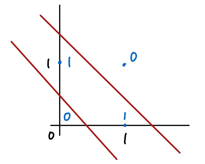
위와 같이 XOR 문제는 선을 2개 그어 문제를 해결할 수 있는데, 한동안 MLP를 현실적으로 학습할 수 있는 방법을 찾지 못하다가 backpropagation이 등장하면서 힉습이 가능해졌다.

---

Data and Model

import torch

device = 'cuda' if torch.cuda.is_available() else 'cpu'

# 시드 고정
torch.manual_seed(777)
if device == 'cuda':
    torch.cuda.manual_seed_all(777)

X = torch.FloatTensor([[0, 0], [0, 1], [1, 0], [1, 1]]).to(device)
Y = torch.FloatTensor([[0], [1], [1], [0]]).to(device)

위와 같이 데이터를 XOR에 맞게 만들어 주고, 모델도 생성해 준다. 이번에는 MLP로 학습할 것이기 때문에 선형 레이어 2개를 만들어 Sequential로 묶어 준다. loss는 마찬가지로 이진분류이므로 BCELoss를 사용한다.

linear1 = torch.nn.Linear(2, 2, bias=True)
linear2 = torch.nn.Linear(2, 1, bias=True)
sigmoid = torch.nn.Sigmoid()

model = torch.nn.Sequential(linear1, sigmoid, linear2, sigmoid).to(device)

criterion = torch.nn.BCELoss().to(device)
optimizer = torch.optim.SGD(model.parameters(), lr=1)

---

Train

학습 코드의 형태는 동일하다.

for step in range(10001):
    hypothesis = model(X)

    # cost/loss function
    cost = criterion(hypothesis, Y)

    optimizer.zero_grad()
    cost.backward()
    optimizer.step()

    if step % 100 == 0:
        print(step, cost.item())

'''output
0 0.7434073090553284
100 0.6931650638580322
200 0.6931577920913696
300 0.6931517124176025
400 0.6931463479995728
500 0.6931411027908325
600 0.693135678768158
700 0.6931295394897461
800 0.693122148513794
900 0.6931126713752747
1000 0.6930999755859375
...
9700 0.001285637030377984
9800 0.0012681199004873633
9900 0.0012511102249845862
10000 0.0012345188297331333
'''

조금씩이지만 확실히 loss가 줄어드는 것을 확인할 수 있다. 정확도도 한번 출력해 보자.

with torch.no_grad():
    hypothesis = model(X)
    predicted = (hypothesis > 0.5).float()
    accuracy = (predicted == Y).float().mean()
    print('\nHypothesis: ', hypothesis.detach().cpu().numpy(), '\nCorrect: ', predicted.detach().cpu().numpy(), '\nAccuracy: ', accuracy.item())

'''output

Hypothesis:  [[0.00106364]
 [0.99889404]
 [0.99889404]
 [0.00165861]] 
Correct:  [[0.]
 [1.]
 [1.]
 [0.]] 
Accuracy:  1.0
'''

XOR을 아주 잘 분류해 준다. 이번 학습에서는 2개의 레이어만을 쌓았지만 여러개의 레이어, 또는 더 노드가 많은 레이어도 만들 수 있다.

NN Wide Deep

linear1 = torch.nn.Linear(2, 10, bias=True)
linear2 = torch.nn.Linear(10, 10, bias=True)
linear3 = torch.nn.Linear(10, 10, bias=True)
linear4 = torch.nn.Linear(10, 1, bias=True)
sigmoid = torch.nn.Sigmoid()

model = torch.nn.Sequential(linear1, sigmoid, linear2, sigmoid, linear3, sigmoid, linear4, sigmoid).to(device)

for step in range(10001):
    optimizer.zero_grad()
    hypothesis = model(X)

    # cost/loss function
    cost = criterion(hypothesis, Y)
    cost.backward()
    optimizer.step()

    if step % 100 == 0:
        print(step, cost.item())

'''output
0 0.6948983669281006
100 0.6931558847427368
200 0.6931535005569458
300 0.6931513547897339
400 0.6931493282318115
500 0.6931473016738892
600 0.6931453943252563
700 0.6931434869766235
800 0.6931416988372803
900 0.6931397914886475
1000 0.6931380033493042
...
9700 0.00016829342348501086
9800 0.00016415018762927502
9900 0.00016021561168599874
10000 0.0001565046259202063
'''

2개의 레이어를 쌓았을 때(0.0012345188297331333)보다 loss가 더 낮아진 것을 확인할 수 있다.