카테고리: pytorch

def evaluate(pairs, source_vocab, target_vocab, encoder, decoder, target_max_length):
    for pair in pairs:
        print(">", pair[0])
        print("=", pair[1])
        source_tensor = tensorize(source_vocab, pair[0])
        source_length = source_tensor.size()[0]
        encoder_hidden = torch.zeros([1, 1, encoder.hidden_size]).to(device)

        for ei in range(source_length):
            _, encoder_hidden = encoder(source_tensor[ei], encoder_hidden)

        decoder_input = torch.Tensor([[SOS_token]]).long().to(device) # 수정해야 작동
        decoder_hidden = encoder_hidden
        decoded_words = []

        for di in range(target_max_length):
            decoder_output, decoder_hidden = decoder(decoder_input, decoder_hidden)
            _, top_index = decoder_output.data.topk(1) # 1개의 가장 큰 요소를 반환
            if top_index.item() == EOS_token:
                decoded_words.append("<EOS>")
                break
            else:
                decoded_words.append(target_vocab.index2vocab[top_index.item()])

            decoder_input = top_index.squeeze().detach()

        predict_words = decoded_words
        predict_sentence = " ".join(predict_words)
        print("<", predict_sentence)
        print("")

# load data
xy = np.loadtxt("data-02-stock_daily.csv", delimiter=",")
xy = xy[::-1]  # reverse order

# split train-test set
train_size = int(len(xy) * 0.7)
train_set = xy[0:train_size]
test_set = xy[train_size - seq_length:]

앞서 언급한대로 scaling을 하고 학습하기 좋은 형태로 data를 가공해야 한다.

def minmax_scaler(data):
    numerator = data - np.min(data, 0)
    denominator = np.max(data, 0) - np.min(data, 0)
    return numerator / (denominator + 1e-7)

train_set = minmax_scaler(train_set)
test_set = minmax_scaler(test_set)

# data setting
x_data = []
y_data = []

# window를 오른쪽으로 움직이면서 자름
for i in range(0, len(sentence) - sequence_length):
    x_str = sentence[i:i + sequence_length]
    y_str = sentence[i + 1: i + sequence_length + 1]
    print(i, x_str, '->', y_str)

    x_data.append([char_dic[c] for c in x_str])  # x str to index (dict 사용)
    y_data.append([char_dic[c] for c in y_str])  # y str to index

x_one_hot = [np.eye(dic_size)[x] for x in x_data]

X = torch.FloatTensor(x_one_hot)
Y = torch.LongTensor(y_data)

'''output
0 if you wan -> f you want
1 f you want ->  you want 
2  you want  -> you want t
3 you want t -> ou want to
4 ou want to -> u want to 
...
166 ty of the  -> y of the s
167 y of the s ->  of the se
168  of the se -> of the sea
169 of the sea -> f the sea.
'''

char_set = ['h', 'i', 'e', 'l', 'o']

# hyper parameters
input_size = len(char_set)
hidden_size = len(char_set)
learning_rate = 0.1

# data setting
x_data = [[0, 1, 0, 2, 3, 3]]
x_one_hot = [[[1, 0, 0, 0, 0],
              [0, 1, 0, 0, 0],
              [1, 0, 0, 0, 0],
              [0, 0, 1, 0, 0],
              [0, 0, 0, 1, 0],
              [0, 0, 0, 1, 0]]]
y_data = [[1, 0, 2, 3, 3, 4]]

X = torch.FloatTensor(x_one_hot)
Y = torch.LongTensor(y_data)

마찬가지로 one-hot encoding하여 Tensor로 바꾼다. 다만 각 알파벳 변수에 배열을 저장하는 방식이 아니라 char_set에 저장된 알파벳을 x_data의 값을 인덱스로 불러오는 방식이다. one-hot encoding은 x_data에 적용하여 학습한다.

rnn = torch.nn.RNN(input_size, hidden_size)

outputs, _status = rnn(input_data)
print(outputs)
print(outputs.size())

'''output
tensor([[[-0.7497, -0.6135],
         [-0.5282, -0.2473],
         [-0.9136, -0.4269],
         [-0.9136, -0.4269],
         [-0.9028,  0.1180]],

        [[-0.5753, -0.0070],
         [-0.9052,  0.2597],
         [-0.9173, -0.1989],
         [-0.9173, -0.1989],
         [-0.8996, -0.2725]],

        [[-0.9077, -0.3205],
         [-0.8944, -0.2902],
         [-0.5134, -0.0288],
         [-0.5134, -0.0288],
         [-0.9127, -0.2222]]], grad_fn=<StackBackward>)
torch.Size([3, 5, 2])
'''

activation과 weight를 명시하여 표현하면 다음과 같다.

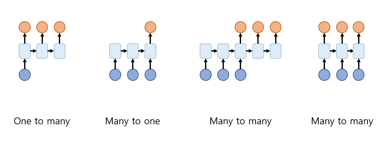
이런 RNN의 구조를 응용하여 다음과 같은 구조들로 사용할 수 있다.

• one to many : 하나의 입력을 받아 여러 출력을 내는 구조이다. 하나의 이미지를 받아 그에 대한 설명을 문장(여러개의 단어)으로 출력하는 것을 예로 들 수 있다.

• many to one : 여러 입력을 받아 하나의 출럭을 내는 구조이다. 문장을 입력받아 그 문장이 나타내는 감정의 label을 출력하는 것을 예로 들 수 있다.

• many to many : 2가지의 구조가 있는 것을 볼 수 있다.

  • 입력이 다 끝나는 지점부터 여러 출력을 내는 구조로, 문장을 입력받아 번역하는 모델을 예로 들 수 있다. 이 경우 문장의 중간에 번역을 진행하면 다 끝나고 나서 문장의 의미가 달라질 수 있기 때문에 먼저 입력 문장을 다 듣고 번역을 진행하게 된다.
  • 입력 하나하나를 받으면서 그때마다 모델의 출력을 내는 구조이다. 영상을 처리할 때 frame 단위의 이미지로 나눠 입력을 받은 후 각 frame을 입력 받을 때마다 처리하는 것을 예로 들 수 있다.

    # self.inplanes = 64
    # self.layer1 = self._make_layer(block=Bottleneck, 64, layers[0]=3)
    def _make_layer(self, block, planes, blocks, stride=1):
        
        downsample = None
        
        # identity 값을 낮춰서 shape을 맞춰주기 위함. channel도 맞춰주기.
        if stride != 1 or self.inplanes != planes * block.expansion: # 64 != 64 * 4
            
            downsample = nn.Sequential(
                conv1x1(self.inplanes, planes * block.expansion, stride), #conv1x1(256, 512, 2) #conv1x1(64, 256, 2)
                nn.BatchNorm2d(planes * block.expansion), #batchnrom2d(512) #batchnrom2d(256)
            )

        layers = []
        layers.append(block(self.inplanes, planes, stride, downsample))
        # layers.append(Bottleneck(64, 64, 1, downsample))
        
        self.inplanes = planes * block.expansion #self.inplanes = 128 * 4
        
        for _ in range(1, blocks): 
            layers.append(block(self.inplanes, planes)) # * 3

        return nn.Sequential(*layers)

criterion = nn.CrossEntropyLoss().to(device)
optimizer = torch.optim.SGD(vgg16.parameters(), lr = 0.005,momentum=0.9)

# 학습이 진행됨에 따라 lr 조절
lr_sche = optim.lr_scheduler.StepLR(optimizer, step_size=5, gamma=0.9) # optimizer의 step이 5번 진행될 때마다 gamma만큼 곱함

기존과 다른 점은 학습된 정도에 따라 learning rate를 줄이는 코드가 추가되었다는 것이다.

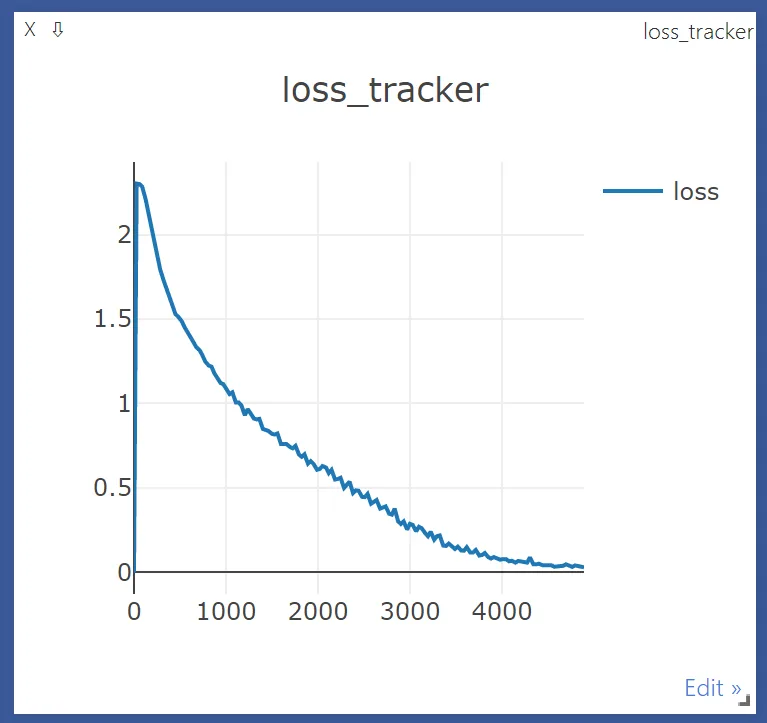
lr_sche.step()이 추가된 것 말고 크게 다른 점은 없다.

correct = 0
total = 0

with torch.no_grad():
    for data in testloader:
        images, labels = data
        images = images.to(device)
        labels = labels.to(device)
        outputs = vgg16(images)
        
        _, predicted = torch.max(outputs.data, 1)
        
        total += labels.size(0)
        
        correct += (predicted == labels).sum().item()

print('Accuracy of the network on the 10000 test images: %d %%' % (
    100 * correct / total))

Accuracy of the network on the 10000 test images: 75 %

import torchvision
from torchvision import transforms

from torch.utils.data import DataLoader

from matplotlib.pyplot import imshow
%matplotlib inline

trans = transforms.Compose([
    transforms.Resize((64,128))
])

train_data = torchvision.datasets.ImageFolder(root='custom_data/origin_data', transform=trans)

원본 데이터가 있는 곳을 root로 잡고 Compose를 통해 적용할 transforms들을 묶어 넣어준다. 원본 데이터가 265x512로 너무 커서 64x128로 바꾸어주는 과정을 거친다. 여기서는 하나의 transforms을 사용하지만 어러개를 사용해야할 때 Compose로 묶어 사용할 수 있다.