모두를 위한 딥러닝 2 - Lab7-2: MNIST Intoduction
모두를 위한 딥러닝 Lab7-2: MNIST Intoduction 강의를 본 후 공부를 목적으로 작성한 게시물입니다.
MNIST dataset
MNIST 데이터 셋은 숫자 손글씨를 모아놓은 데이터 셋이다. 사람들이 적은 숫자들을 우체국에서 자동으로 처리하기 위해 만들어진 것이 이 셋의 시작점이라고 한다.
MNIST는 다음과 같이 28x28 크기의 픽셀, 1개의 gray channel 그리고 0 ~ 9의 정수 label로 이루어져 있다.
torchvision
minist는 torchvision 모듈을 통해 불러온다. torchvision은 여러 데이터 셋이나 아키텍처, 전처리를 할 수 있는 기능들을 내장하고 있는 모듈이다.
1
2
3
4
5
6
7
8
9
10
11
12
13
14
15
16
17
18
19
20
21
22
import torch
import torchvision.datasets as dsets
import torchvision.transforms as transforms
import matplotlib.pyplot as plt

# parameters
training_epochs = 15
batch_size = 100

# MNIST dataset
mnist_train = dsets.MNIST(root='MNIST_data/',
                          train=True, # train set
                          transform=transforms.ToTensor(),
                          download=True)

mnist_test = dsets.MNIST(root='MNIST_data/',
                         train=False, # test set
                         transform=transforms.ToTensor(),
                         download=True)

# minibatch
data_loader - torch.utils.DataLoader(DataLoader=mnist_train, batch_size=batch_size, shuffle=True, drop_last=True)
mnist는 60000개의 train set과 10000개의 test set으로 구성되어 있고, train prameter에 boolean 값을 넣어 각 셋을 불러올 수 있다.
다른 데이터 셋들과 마찬가지로 DataLoader를 통해 미니배치를 나누어 학습할 수 있다.
Model
1
2
3
4
5
6
# MNIST data image of shape 28 * 28 = 784
linear = torch.nn.Linear(784, 10, bias=True).to(device)

# define cost/loss & optimizer
criterion = torch.nn.CrossEntropyLoss().to(device)
optimizer = torch.optim.SGD(linear.parameters(), lr=0.1)
모델은 선형모델을 사용하며 이미지의 크기가 28x28이므로 28*28=784의 차원을 가지는 입력을 받도록 정의한다.
Train
1
2
3
4
5
6
7
8
9
10
11
12
13
14
15
16
17
18
19
20
21
22
23
24
25
26
27
28
29
30
31
32
33
34
35
36
37
38
39
40
41
for epoch in range(training_epochs):
    avg_cost = 0
    total_batch = len(data_loader)

    for X, Y in data_loader:
        # reshape input image into [batch_size by 784]
        # label is not one-hot encoded
        X = X.view(-1, 28 * 28).to(device)
        Y = Y.to(device)

        hypothesis = linear(X)
        cost = criterion(hypothesis, Y)

        optimizer.zero_grad()
        cost.backward()
        optimizer.step()

        avg_cost += cost / total_batch

    print('Epoch:', '%04d' % (epoch + 1), 'cost =', '{:.9f}'.format(avg_cost))

print('Learning finished')

'''output
Epoch: 0001 cost = 0.535468459
Epoch: 0002 cost = 0.359274179
Epoch: 0003 cost = 0.331187516
Epoch: 0004 cost = 0.316578031
Epoch: 0005 cost = 0.307158142
Epoch: 0006 cost = 0.300180674
Epoch: 0007 cost = 0.295130163
Epoch: 0008 cost = 0.290851504
Epoch: 0009 cost = 0.287417084
Epoch: 0010 cost = 0.284379542
Epoch: 0011 cost = 0.281825215
Epoch: 0012 cost = 0.279800713
Epoch: 0013 cost = 0.277809024
Epoch: 0014 cost = 0.276154280
Epoch: 0015 cost = 0.274440825
Learning finished
'''
Lab4-2에서 학습한 방식과 같이 data_loader를 for를 통해 반복하며 진행한다.
이때 기존의 이미지 데이터의 minibatch는 [batch_size, 1, 28, 28]의 크기를 가지기 때문에, 모델의 입력에 맞게 [batch_size, 28*28]로 바꿔주는 과정이 필요하다. 이 과정을 위해 X = X.view(-1, 28 * 28).to(device)로 데이터를 재구성한 것을 볼 수 있다.
나머지는 학습은 기존의 형태와 동일하다.
Test
테스트를 진행할 때에는 이미 학습된 모델에 대해 학습이 잘 되었는지를 확인하는 것이기 때문에 gradient descent로 인한 가중치 업데이트가 되면 안된다. 그래서 with torch.no_grad() 안에서 업데이트 되는 것을 막으면서 테스트를 진행한다.
1
2
3
4
5
6
7
8
9
10
11
12
13
14
15
16
17
18
19
20
21
22
23
24
25
26
27
# Test the model using test sets
with torch.no_grad():
X_test = mnist_test.test_data.view(-1, 28 * 28).float().to(device)
Y_test = mnist_test.test_labels.to(device)
prediction = linear(X_test)
correct_prediction = torch.argmax(prediction, 1) == Y_test
accuracy = correct_prediction.float().mean()
print('Accuracy:', accuracy.item())
# Get one and predict
r = random.randint(0, len(mnist_test) - 1)
X_single_data = mnist_test.test_data[r:r + 1].view(-1, 28 * 28).float().to(device)
Y_single_data = mnist_test.test_labels[r:r + 1].to(device)
print('Label: ', Y_single_data.item())
single_prediction = linear(X_single_data)
print('Prediction: ', torch.argmax(single_prediction, 1).item())
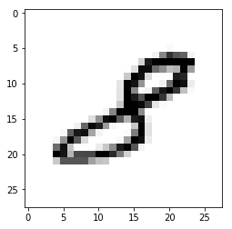
plt.imshow(mnist_test.test_data[r:r + 1].view(28, 28), cmap='Greys', interpolation='nearest')
plt.show()
'''output
Accuracy: 0.8862999677658081
Label: 8
Prediction: 3
'''
학습한 모델에 test 입력을 통과시켜 나온 결과를 argmax를 통해 모델이 예측한 label을 뽑아낼 수 있다. 이후 test의 실제 label과 비교하여 ByteTensor를 생성하고, 그 평균을 구해 정확도를 계산할 수 있다.
한 데이터에 대한 출력값은 싶다면 test_data와 label을 슬라이싱 하여 모델에 넣어서 결과값을 출력하는 것으로 확인할 수 있다.
그 데이터에 대한 이미지는 plt.imshow를 통해 롹인할 수 있다. cmap(color map)을 grey로 설정하고, interpolation(보간)을 nearest로 하면 mnist 이미지를 얻을 수 있다.