모두를 위한 딥러닝 2 - Lab10-6: ResNet
모두를 위한 딥러닝 Lab10-6: Advence CNN(ResNet) 강의를 본 후 공부를 목적으로 작성한 게시물입니다.
Plain Network
Plain network는 skip connection을 사용하지 않은 일반적인 CNN 신경망을 의미한다. 이러한 plain net이 깊어지면 깊어질수록 backpropagation을 할 때 기울기 소실이나 폭발이 발생할 확률이 높아진다.
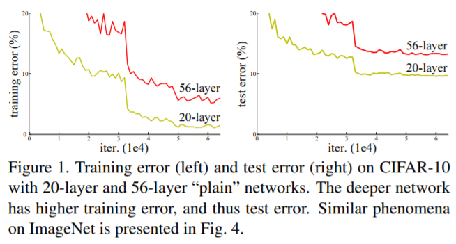
위 그래프에서도 확인할 수 있듯이 plain network를 깊게 쌓은 것이 오히려 학습이 잘 안 된 것을 볼 수 있다. 이는 너무 깊은 plain network에서 기울기 소실 혹은 폭발이 발생하여 원래 원하던 방향으로 학습이 안되었기 때문이다.
Identity Mapping
Classification problem에서 모델이 완벽하게 학습하였다면 input($x$)과 output(y)의 의미는 같아야 한다. (강아지 이미지면 강아지 categry) 이 말은 $H(x)$가 $x$가 되도록 학습하면 된다는 것이다. 즉, $H(x)=x$가 되도록 학습을 한다는 것이며 이는 일종의 항등함수(identity function)이므로, Classification problem의 model을 최적화 한다는 것은 identity mapping을 학습하는 것과 같아진다.
ResNet
ResNet은 skip connection을 적용한 network로 기울기 소실을 해결하면서 layer를 더 깊게 쌓아 성능이 좋은 모델을 구성할 수 있다.
Skip(Shortcut) Connection
기존의 network에서는 input ($x$)를 target ($y$)로 mapping(identity mapping)하는 $H(x)$를 얻는 것이 목적이었다. 하지만 identity mapping을 통해 학습을 진행해도 layer가 쌓일수록 기울기 소실이 발생하는 것은 어쩔 수 없다.
이를 해결하기위해 제안한 방법론이 Residual learning이다. 이는 $H(x)$를 직접 학습하는 것이 아닌 잔차(residual), $F(x) = H(x)-x$를 최소화하는 것을 목표로 하는 방법이다. 이 잔차 $F(x)$를 최소화 하면 $H(x) = x$에 가까운 이상적인 모델을 찾을 수 있다는 발상이다.
이 방법론이 제안된 전제는 residual mapping이 그냥 identity mapping하는 방식보다 최적화하기 쉽다이다. 즉, 직접 $H(x)=x$를 목적으로 학습하는 것 보다는 현재 block의 input(이전 block의 output)의 정보($x$, identity)를 지닌 채 추가적으로 학습하는 것이 더 쉬운 학습이 된다는 것이다.
또한, output에 $x$를 더해주게 되면 미분을 해도 $x$의 미분값은 1이기 때문에 각 layer들은 최소 1의 미분값을 지니게 되어 앞서 문제였던 기울기 소실 문제가 해결된다.
이런 network를 구성하기 위해 아래의 구조와 같이 여러 layer를 건너뛰어(skip) 한 layer의 output을 다음 layer의 input에 더해주는 구조를 만들었다. identity가 다음 output으로 가는 지름길(shortcut)을 만들어 주었다고 해서 shortcut connection이라고도 한다.
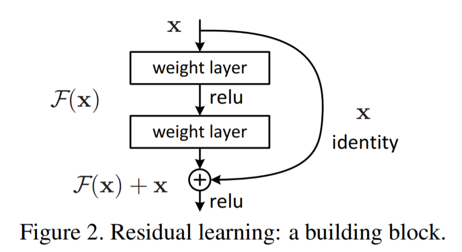
이렇게 skip connection이 적용된 부분을 residual block이라고 한다.
Bottleneck Block
Residual block애서 중간 layer를 1x1 -> 3x3 -> 1x1 의 bottleneck 구조를 만들어 demension redeuction을 통해 연산 시간을 줄인 구조이다.

고정된 layer들을 제외하면 크게 4개의 layer가 있는 것을 볼 수 있는데, VGG와 비슷하게 3x3 conv에 padding 1을 적용하여 하나의 큰 layer안에서는 ourput size가 고정되는 것을 볼 수 있다.
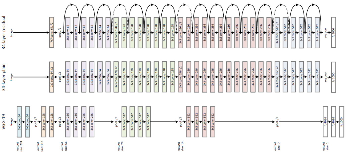
그림으로 보면 위와 같은 구조를 지니고 있다. VGG 구조보다 확실히 깊은 구조인 것을 확인할 수 있다.
Code with ResNet
PyTorch의 Resnet을 뜯어보자.
BasicBlock
먼저 residual block이다.
1
2
3
4
5
6
7
8
9
10
11
12
13
14
15
16
17
18
19
20
21
22
23
24
25
26
27
28
29
30
31
32
33
class BasicBlock(nn.Module):
    expansion = 1

    def __init__(self, inplanes, planes, stride=1, downsample=None):
        super(BasicBlock, self).__init__()
        self.conv1 = conv3x3(inplanes, planes, stride)
        self.bn1 = nn.BatchNorm2d(planes)
        self.relu = nn.ReLU(inplace=True)
        self.conv2 = conv3x3(planes, planes)
        self.bn2 = nn.BatchNorm2d(planes)
        self.downsample = downsample
        self.stride = stride

    def forward(self, x):
        # x.shape = 3, 64, 64
        identity = x
        # identity = 3, 64, 64
        out = self.conv1(x) # 3x3 stride = stride = 2
        out = self.bn1(out)
        out = self.relu(out)
        # out.shape = 3, 32, 32
        out = self.conv2(out) # 3x3 stride = 1
        # out.shape = 3, 32, 32
        out = self.bn2(out)
        # out.shape = 3, 32, 32
        # identity = 3, 64, 64 -> 덧셈 불가
        if self.downsample is not None:
            identity = self.downsample(x)

        out += identity
        out = self.relu(out)

        return out
앞서 살펴봤던 residual block의 구조와 다르지 않은 모습이다. 2개의 3x3 conv layer를 통과하고 마지막에 입력인 identity를 더해준 후 output을 내어주는 형태이다.
다만 다른 점이 있다면 downsample이 있는 것인데, 이는 주석으로 처리된 예시로 설명이 된다. 만약 3x64x64의 입력이 들어오고 conv1의 stride를 2로 한다면 identity를 더하기 전의 out.shape이 3x32x32로 기존과 달라지게 되어 identity와의 덧셈이 불가능해진다. 이 경우 identity를 downsample하여 shape을 맞춰준다. 그래서 만약 stride에 따라 out의 shape이 달라지게 되는 경우 downsample 옵션을 주어 shape을 맞춰야 한다.
Bottleneck
1
2
3
4
5
6
7
8
9
10
11
12
13
14
15
16
17
18
19
20
21
22
23
24
25
26
27
28
29
30
31
32
33
34
35
36
37
38
39
40
41
42
43
44
45
46
def conv3x3(in_planes, out_planes, stride=1):
    """3x3 convolution with padding"""
    return nn.Conv2d(in_planes, out_planes, kernel_size=3, stride=stride,
                     padding=1, bias=False)


def conv1x1(in_planes, out_planes, stride=1):
    """1x1 convolution"""
    return nn.Conv2d(in_planes, out_planes, kernel_size=1, stride=stride, bias=False)

class Bottleneck(nn.Module):
    expansion = 4

    def __init__(self, inplanes, planes, stride=1, downsample=None):
        super(Bottleneck, self).__init__()
        self.conv1 = conv1x1(inplanes, planes)
        self.bn1 = nn.BatchNorm2d(planes)
        self.conv2 = conv3x3(planes, planes, stride)
        self.bn2 = nn.BatchNorm2d(planes)
        self.conv3 = conv1x1(planes, planes * self.expansion)
        self.bn3 = nn.BatchNorm2d(planes * self.expansion)
        self.relu = nn.ReLU(inplace=True)
        self.downsample = downsample
        self.stride = stride

    def forward(self, x):
        identity = x

        out = self.conv1(x) # 1x1 stride = 1
        out = self.bn1(out)
        out = self.relu(out)

        out = self.conv2(out) # 3x3 stride = stride
        out = self.bn2(out)
        out = self.relu(out)

        out = self.conv3(out) # 1x1 stride = 1
        out = self.bn3(out)

        if self.downsample is not None:
            identity = self.downsample(x)

        out += identity
        out = self.relu(out)

        return out
3x3 / 1x1 conv를 따로 정의하여 모델에 사용하고 있는 모습이다. 이 때도 같은 이유로 downsample 옵션이 있다.
ResNet
위의 block class들을 이용해 network를 구성할 차례이다.
_make_layer
먼저 layer를 만들어주는 함수부터 보자.
1
2
3
4
5
6
7
8
9
10
11
12
13
14
15
16
17
18
19
20
21
22
23
24
    # self.inplanes = 64
    # self.layer1 = self._make_layer(block=Bottleneck, 64, layers[0]=3)
    def _make_layer(self, block, planes, blocks, stride=1):

        downsample = None

        # identity 값을 낮춰서 shape을 맞춰주기 위함. channel도 맞춰주기.
        if stride != 1 or self.inplanes != planes * block.expansion: # 64 != 64 * 4

            downsample = nn.Sequential(
                conv1x1(self.inplanes, planes * block.expansion, stride), #conv1x1(256, 512, 2) #conv1x1(64, 256, 2)
                nn.BatchNorm2d(planes * block.expansion), #batchnrom2d(512) #batchnrom2d(256)
            )

        layers = []
        layers.append(block(self.inplanes, planes, stride, downsample))
        # layers.append(Bottleneck(64, 64, 1, downsample))

        self.inplanes = planes * block.expansion #self.inplanes = 128 * 4

        for _ in range(1, blocks):
            layers.append(block(self.inplanes, planes)) # * 3

        return nn.Sequential(*layers)
stride가 1이 아니거나 input과 output의 shape이 맞지 않을 경우 downsample을 conv1x1을 이용하여 shape을 맞출 수 있게 설정해준다.
다음부터는 layer의 크기에 맞게 layer를 block 개수 만큼 만들어 쌓은 후에 반환한다. 주석의 입력 에시를 통해 따라가 보면 이해에 조금 도움이 될 것 같다.
init
1
2
3
4
5
6
7
8
9
10
11
12
13
14
15
16
17
18
19
20
21
22
23
24
25
26
27
28
29
30
31
32
33
34
35
36
37
38
39
40
41
42
    # model = ResNet(Bottleneck, [3, 4, 6, 3], **kwargs) => resnet 50
    def __init__(self, block, layers, num_classes=1000, zero_init_residual=False):
        super(ResNet, self).__init__()

        self.inplanes = 64

        self.conv1 = nn.Conv2d(3, 64, kernel_size=7, stride=2, padding=3, bias=False)

        # outputs = self.conv1(inputs)
        # outputs.shape = 64, 112, 112

        self.bn1 = nn.BatchNorm2d(64)
        self.relu = nn.ReLU(inplace=True)

        # inputs = 64, 112, 112
        self.maxpool = nn.MaxPool2d(kernel_size=3, stride=2, padding=1)
        # output = 64, 56, 56

        self.layer1 = self._make_layer(block, 64, layers[0]'''3''')
        self.layer2 = self._make_layer(block, 128, layers[1]'''4''', stride=2)
        self.layer3 = self._make_layer(block, 256, layers[2]'''6''', stride=2)
        self.layer4 = self._make_layer(block, 512, layers[3]'''3''', stride=2)

        self.avgpool = nn.AdaptiveAvgPool2d((1, 1))
        self.fc = nn.Linear(512 * block.expansion, num_classes)

        for m in self.modules(): # weight init
            if isinstance(m, nn.Conv2d):
                nn.init.kaiming_normal_(m.weight, mode='fan_out', nonlinearity='relu')
            elif isinstance(m, nn.BatchNorm2d):
                nn.init.constant_(m.weight, 1)
                nn.init.constant_(m.bias, 0)

        # Zero-initialize the last BN in each residual branch,
        # so that the residual branch starts with zeros, and each residual block behaves like an identity.
        # This improves the model by 0.2~0.3% according to https://arxiv.org/abs/1706.02677
        if zero_init_residual:
            for m in self.modules():
                if isinstance(m, Bottleneck):
                    nn.init.constant_(m.bn3.weight, 0)
                elif isinstance(m, BasicBlock):
                    nn.init.constant_(m.bn2.weight, 0)
이전에 만들었던 함수들을 모두 사용하여 network를 만든다. 먼저 고정적으로 들어갈 7x7 conv와 maxpooling layer를 만들어준다.
다음으로는 _make_layer를 통해 입력한 layer 개수에 맞게 layer를 생성한다. 마지막으로 1x1로 average pooling을 하고 class 개수에 맞춰 fc layer를 통과시키면 모든 학습이 끝나게 된다.
가중치의 초기화는 conv의 경우 'fan_out' mode의 kaiming_normal_를 사용하고, bn(batch normalize)의 경우 wieght를 1, bias를 0으로 초기화한다. zero_init_residual옵션을 주면 특정 layer의 wieght를 0으로 초기화하는데 이는 해당 논문에서 이 시행을 적용하였더니 성능이 0.2~0.3% 올랐다고 해서 들어가 있는 옵션이라고 한다.
forward
1
2
3
4
5
6
7
8
9
10
11
12
13
14
15
16
    def forward(self, x):
        x = self.conv1(x)
        x = self.bn1(x)
        x = self.relu(x)
        x = self.maxpool(x)

        x = self.layer1(x)
        x = self.layer2(x)
        x = self.layer3(x)
        x = self.layer4(x)

        x = self.avgpool(x)
        x = x.view(x.size(0), -1)
        x = self.fc(x)

        return x
forward에서는 지금까지 만들었던 모델들을 순서대로 이어서 학습되도록 한다.
ResNet Models
1
2
3
4
5
6
7
8
9
10
11
def resnet18(pretrained=False, **kwargs):
    model = ResNet(BasicBlock, [2, 2, 2, 2], **kwargs) #=> 2*(2+2+2+2) +1(conv1) +1(fc)  = 16 +2 =resnet 18
    return model

def resnet50(pretrained=False, **kwargs):
    model = ResNet(Bottleneck, [3, 4, 6, 3], **kwargs) #=> 3*(3+4+6+3) +(conv1) +1(fc) = 48 +2 = 50
    return model

def resnet152(pretrained=False, **kwargs):
    model = ResNet(Bottleneck, [3, 8, 36, 3], **kwargs) # 3*(3+8+36+3) +2 = 150+2 = resnet152
    return mode
위와 같은 방법으로 여러 resnet을 만들어 사용할 수 있다.
하지만 이미 module로 다 만들어져 있기 때문에 아래와 같이 만들어진 것을 사용해서 model을 생성해도 정상적으로 생성되는 것을 확인할 수 있다.
1
2
3
4
5
6
7
8
9
10
11
12
13
14
15
16
17
18
19
20
21
22
23
24
25
26
27
28
29
30
31
32
33
34
35
36
37
38
import torchvision.models.resnet as resnet

res = resnet.resnet50()
res

'''ourput
ResNet(
  (conv1): Conv2d(3, 64, kernel_size=(7, 7), stride=(2, 2), padding=(3, 3), bias=False)
  (bn1): BatchNorm2d(64, eps=1e-05, momentum=0.1, affine=True, track_running_stats=True)
  (relu): ReLU(inplace=True)
  (maxpool): MaxPool2d(kernel_size=3, stride=2, padding=1, dilation=1, ceil_mode=False)
  (layer1): Sequential(
    (0): Bottleneck(
      (conv1): Conv2d(64, 64, kernel_size=(1, 1), stride=(1, 1), bias=False)
      (bn1): BatchNorm2d(64, eps=1e-05, momentum=0.1, affine=True, track_running_stats=True)
      (conv2): Conv2d(64, 64, kernel_size=(3, 3), stride=(1, 1), padding=(1, 1), bias=False)
      (bn2): BatchNorm2d(64, eps=1e-05, momentum=0.1, affine=True, track_running_stats=True)
      (conv3): Conv2d(64, 256, kernel_size=(1, 1), stride=(1, 1), bias=False)
      (bn3): BatchNorm2d(256, eps=1e-05, momentum=0.1, affine=True, track_running_stats=True)
      (relu): ReLU(inplace=True)
      (downsample): Sequential(
        (0): Conv2d(64, 256, kernel_size=(1, 1), stride=(1, 1), bias=False)
        (1): BatchNorm2d(256, eps=1e-05, momentum=0.1, affine=True, track_running_stats=True)
      )
    )
    (1): Bottleneck(
      (conv1): Conv2d(256, 64, kernel_size=(1, 1), stride=(1, 1), bias=False)
      (bn1): BatchNorm2d(64, eps=1e-05, momentum=0.1, affine=True, track_running_stats=True)
      (conv2): Conv2d(64, 64, kernel_size=(3, 3), stride=(1, 1), padding=(1, 1), bias=False)
      (bn2): BatchNorm2d(64, eps=1e-05, momentum=0.1, affine=True, track_running_stats=True)
      (conv3): Conv2d(64, 256, kernel_size=(1, 1), stride=(1, 1), bias=False)
...
    )
  )
  (avgpool): AdaptiveAvgPool2d(output_size=(1, 1))
  (fc): Linear(in_features=2048, out_features=1000, bias=True)
)
'''
Train with ResNet
VGG를 통해 학습했을 때와 마찬가지로 CIFAR10 data를 사용하여 학습을 진행한다.
Data
대부분 VGG 학습할 때와 같다. 다만 다른 부분은 실제 data의 평균과 분산을 구해서 normalize를 진행한다.
1
2
3
4
5
6
7
8
9
10
11
12
13
14
15
16
17
18
19
20
21
22
23
24
25
26
27
28
29
30
31
32
33
34
35
36
37
38
39
40
41
42
43
44
45
46
transform = transforms.Compose([
    transforms.ToTensor()
])

trainset = torchvision.datasets.CIFAR10(root='./cifar10', train=True, download=True, transform=transform)

print(trainset.data.shape)

# 각 축마다 구해서 normalization
train_data_mean = trainset.data.mean( axis=(0,1,2) )
train_data_std = trainset.data.std( axis=(0,1,2) )


print(train_data_mean)
print(train_data_std)

train_data_mean = train_data_mean / 255
train_data_std = train_data_std / 255

print(train_data_mean)
print(train_data_std)

transform_train = transforms.Compose([
    transforms.RandomCrop(32, padding=4),
    transforms.ToTensor(),
    transforms.Normalize(train_data_mean, train_data_std)
])

transform_test = transforms.Compose([
    transforms.ToTensor(),
    transforms.Normalize(train_data_mean, train_data_std)
])

trainset = torchvision.datasets.CIFAR10(root='./cifar10', train=True,
                                        download=True, transform=transform_train)
trainloader = torch.utils.data.DataLoader(trainset, batch_size=256,
                                          shuffle=True, num_workers=0)

testset = torchvision.datasets.CIFAR10(root='./cifar10', train=False,
                                       download=True, transform=transform_test)

testloader = torch.utils.data.DataLoader(testset, batch_size=256,
                                         shuffle=False, num_workers=0)

classes = ('plane', 'car', 'bird', 'cat',
           'deer', 'dog', 'frog', 'horse', 'ship', 'truck')
Model
이번 강의에서는 pyTorch의 ResNet을 사용하지 않고 위에서 정의한 class를 사용하여 학습을 진행했다. 위에서 만든 class와 함수들을 resnet.py에 저장해주고 import하여 사용한다.
1
2
3
4
5
import resnet/

conv1x1=resnet.conv1x1
Bottleneck = resnet.Bottleneck
BasicBlock= resnet.BasicBlock
각 블록들을 먼저 정의해준다.
1
2
3
4
5
6
7
8
9
10
11
12
13
14
15
16
17
18
19
20
21
22
23
24
25
26
27
28
29
30
31
32
33
34
35
36
37
38
39
40
41
42
43
44
45
46
47
48
49
50
51
52
53
54
55
56
57
58
59
60
61
62
63
64
65
66
67
68
69
70
71
72
73
class ResNet(nn.Module):

    def __init__(self, block, layers, num_classes=1000, zero_init_residual=False):
        super(ResNet, self).__init__()
        self.inplanes = 16
        self.conv1 = nn.Conv2d(3, 16, kernel_size=3, stride=1, padding=1,
                               bias=False)
        self.bn1 = nn.BatchNorm2d(16)
        self.relu = nn.ReLU(inplace=True)
        #self.maxpool = nn.MaxPool2d(kernel_size=3, stride=2, padding=1) => 사이즈 작아서 필요 없음

        self.layer1 = self._make_layer(block, 16, layers[0], stride=1)
        self.layer2 = self._make_layer(block, 32, layers[1], stride=1)
        self.layer3 = self._make_layer(block, 64, layers[2], stride=2)
        self.layer4 = self._make_layer(block, 128, layers[3], stride=2)

        self.avgpool = nn.AdaptiveAvgPool2d((1, 1))
        self.fc = nn.Linear(128 * block.expansion, num_classes)

        for m in self.modules():
            if isinstance(m, nn.Conv2d):
                nn.init.kaiming_normal_(m.weight, mode='fan_out', nonlinearity='relu')
            elif isinstance(m, nn.BatchNorm2d):
                nn.init.constant_(m.weight, 1)
                nn.init.constant_(m.bias, 0)

        # Zero-initialize the last BN in each residual branch,
        # so that the residual branch starts with zeros, and each residual block behaves like an identity.
        # This improves the model by 0.2~0.3% according to https://arxiv.org/abs/1706.02677
        if zero_init_residual:
            for m in self.modules():
                if isinstance(m, Bottleneck):
                    nn.init.constant_(m.bn3.weight, 0)
                elif isinstance(m, BasicBlock):
                    nn.init.constant_(m.bn2.weight, 0)

    def _make_layer(self, block, planes, blocks, stride=1):
        downsample = None
        if stride != 1 or self.inplanes != planes * block.expansion:
            downsample = nn.Sequential(
                conv1x1(self.inplanes, planes * block.expansion, stride),
                nn.BatchNorm2d(planes * block.expansion),
            )

        layers = []
        layers.append(block(self.inplanes, planes, stride, downsample))
        self.inplanes = planes * block.expansion
        for _ in range(1, blocks):
            layers.append(block(self.inplanes, planes))

        return nn.Sequential(*layers)

    def forward(self, x):
        x = self.conv1(x)
        #x.shape =[1, 16, 32,32]
        x = self.bn1(x)
        x = self.relu(x)
        #x = self.maxpool(x)

        x = self.layer1(x)
        #x.shape =[1, 128, 32,32]
        x = self.layer2(x)
        #x.shape =[1, 256, 32,32]
        x = self.layer3(x)
        #x.shape =[1, 512, 16,16]
        x = self.layer4(x)
        #x.shape =[1, 1024, 8,8]

        x = self.avgpool(x)
        x = x.view(x.size(0), -1)
        x = self.fc(x)

        return x
정의한 블록들을 사용하여 앞서 구현했던 것과 같이 network를 구성한다. 다만 CIFAR10의 이미지 사이즈가 imagenet보다 작기 때문에 그에 맞게 첫 conv의 kernel size를 3으로 조절해주고, pooling은 없애며, layer의 inplanes도 (64, 128, 256, 512)에서 (16, 32, 64, 128)로 바꿔준다.
이후로 다른 점은 크게 없어 visdom을 통한 결과만 한 번 확인해 보면 다음과 같이 80%의 정확도까지 학습이 된 것을 확인할 수 있다.(20 epoch 진행)
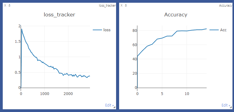
Image Source
- 20-layer vs. 56-layer plain network, Residual Block, ResNet Models Table, Resnet-34 Architecture: https://arxiv.org/pdf/1512.03385.pdf
- Bottleneck Bock: https://icml.cc/2016/tutorials/icml2016_tutorial_deep_residual_networks_kaiminghe.pdf