모두를 위한 딥러닝 2 - Lab10-5: VGG
모두를 위한 딥러닝 Lab10-5: Advence CNN(VGG) 강의를 본 후 공부를 목적으로 작성한 게시물입니다.
VGG-net(Visual Geometry Group-network)
VGG-net(이하 VGG)은 14년도 ILSVRC(Imagenet 이미지 인식 대회)에 나온 네트워크로 옥스포드의 Visual Geometry Group에서 만든 모델이다.
먼저 논문에서 발표한 VGG모델들의 구조를 보자.
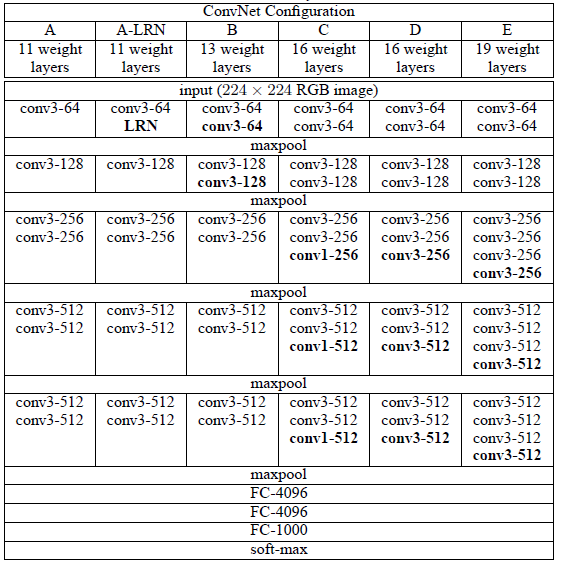
총 6개의 구조를 만들어 성능을 비교하였는데 E로 갈 수록 깊은 모델이며 모델이 깊어질수록 좋은 성능을 보였다고 한다.
VGG는 여러 층에 따라 이름을 붙여주는데 예를 들면 E의 경우 총 19층(16(conv) + 3(fc) = 19)이므로 VGG19이다.
VGG16 Architecture
뒤의 학습에서도 사용할 VGG16의 구조를 대표적으로 확인해보자. Imagenet의 이미지 크기인 224x224에 rgb 3채널의 input을 받는 모델의 구조이다.
구조를 보면 3x3 커널로 여러번의 conv를 진행하는데 그 이유는 훈련해야할 가중치를 줄이기 위해서이다.
224x224 크기의 행렬에 3x3커널로 stride=1 의 conv를 2번 하면 output size는 220x220이고,
\[ Output \, size = \frac{input \, size - filter \, size + (2*padding)}{Stride} + 1 \\
=((224 - 3) + 1)-3 + 1 = 220 \]
5x5 커널로 stride=1 의 conv를 하면 output size는 $224-5+1=220$로 output size가 같은 것을 볼 수 있다. 참고로 3번의 3x3 conv를 하면 7x7 conv 한번과 size가 같다.
같은 output size지만 3x3 conv를 사용한 경우에는 학습해야할 가중치는 $2(3\times3)=18$이고, 5x5의 경우에는 $5\times5=25$로 학습해야할 양이 더 많다. 또한 여러개의 conv 층을 사용할 경우 비선형성이 더 늘어나서 보다 복잡한 데이터를 잘 학습할 수 있다는 장점도 있다.
또 다른 VGG의 특징으로는 conv마다 padding=1을 해줘서 conv 전후의 size를 같게 만들어준다는 것이다. 이런 특성들을 확인하고 VGG16의 구조를 살펴보자.
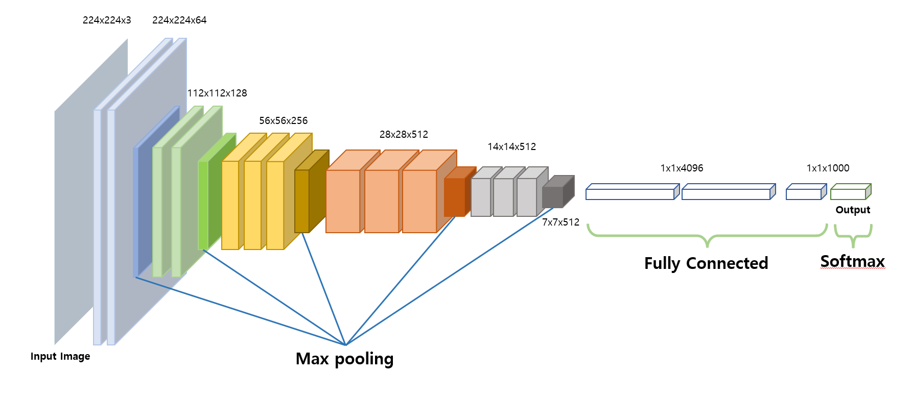
앞서 언급했듯이 3x3 conv를 padding=1로 2~3번 적용하고 max plooing(kernel size=2, stride=2)을 하여 크기를 줄여 다음 conv로 넘겨준다. (이때 activation은 ReLU)
이렇게 conv + max pooling의 큰 layer를 5번 통과하고 나면 data를 platten하게 만들어서 fully connected layer를 통과시킨다. 이때 fully connected layer는 마지막 max pooling의 output size에 맞춰 $7\times7\times512$ 의 input을 받을 수 있게 한다. 마지막 layer에서는 imagenet의 class 개수인 1000으로 맞춰주고 softmax를 적용시킨다.
이를 코드로 풀어 표현하면 다음과 같다.
1
2
3
4
5
6
7
8
9
10
11
12
13
14
15
16
17
18
19
20
21
22
23
24
25
26
27
28
29
30
31
32
33
34
35
36
37
38
39
40
41
42
43
44
45
46
47
48
49
50
conv2d = nn.Conv2d(3, 64, kernel_size=3, padding=1)
nn.ReLU(inplace=True)
conv2d = nn.Conv2d(3, 64, kernel_size=3, padding=1)
nn.ReLU(inplace=True)

nn.MaxPool2d(kernel_size=2, stride=2)

conv2d = nn.Conv2d(64, 128, kernel_size=3, padding=1)
nn.ReLU(inplace=True)
conv2d = nn.Conv2d(128, 128, kernel_size=3, padding=1)
nn.ReLU(inplace=True)

nn.MaxPool2d(kernel_size-2, stride=2)

conv2d = nn.Conv2d(128, 256, kernel_size=3, padding=1)
nn.ReLU(inplace=True)
conv2d = nn.Conv2d(256, 256, kernel_size=3, padding=1)
nn.ReLU(inplace=True)
conv2d = nn.Conv2d(256, 256, kernel_size=3, padding=1)
nn.ReLU(inplace=True)

nn.MaxPool2d(kernel_size=2, stride=2)

conv2d = nn.Conv2d(256, 512, kernel_size=3, padding=1)
nn.ReLU(inplace=True)
conv2d = nn.Conv2d(512, 512, kernel_size=3, padding=1)
nn.ReLU(inplace=True)
conv2d = nn.Conv2d(512, 512, kernel_size=3, padding=1)
nn.ReLU(inplace=True)

nn.MaxPool2d(kernel_size=2, stride=2)

conv2d = nn.Conv2d(512, 512, kernel_size=3, padding=1)
nn.ReLU(inplace=True)
conv2d = nn.Conv2d(512, 512, kernel_size=3, padding=1)
nn.ReLU(inplace=True)
conv2d = nn.Conv2d(512, 512, kernel_size=3, padding=1)
nn.ReLU(inplace=True)

nn.MaxPool2d(kernel_size=2, stride=2)

x = x.view(x.size(0), -1) # flatten

nn.Linear(512 * 7 * 7, 4096),
nn.ReLU(True),
nn.Dropout(),
nn.Linear(4096, 4096),
nn.ReLU(True),
nn.Dropout(),
nn.Linear(4096, 1000),
Code with VGG
PyTorch에 구현된 VGG를 한번 뜯어보자. 먼저 conv layer를 만드는 과정이다.
1
2
3
4
5
6
7
8
9
10
11
12
13
14
15
16
17
18
19
20
21
22
23
24
cfg = {
    'A': [64, 'M', 128, 'M', 256, 256, 'M', 512, 512, 'M', 512, 512, 'M'], #8(conv) + 3(fc) =11 == vgg11
    'B': [64, 64, 'M', 128, 128, 'M', 256, 256, 'M', 512, 512, 'M', 512, 512, 'M'], # 10 + 3 = vgg 13
    'D': [64, 64, 'M', 128, 128, 'M', 256, 256, 256, 'M', 512, 512, 512, 'M', 512, 512, 512, 'M'], #13 + 3 = vgg 16
    'E': [64, 64, 'M', 128, 128, 'M', 256, 256, 256, 256, 'M', 512, 512, 512, 512, 'M', 512, 512, 512, 512, 'M'], # 16 +3 =vgg 19
    'custom' : [64,64,64,'M',128,128,128,'M',256,256,256,'M']
}

def make_layers(cfg, batch_norm=False):
    layers = []
    in_channels = 3

    for v in cfg:
        if v == 'M':
            layers += [nn.MaxPool2d(kernel_size=2, stride=2)]
        else:
            conv2d = nn.Conv2d(in_channels, v, kernel_size=3, padding=1)

            if batch_norm:
                layers += [conv2d, nn.BatchNorm2d(v), nn.ReLU(inplace=True)]
            else:
                layers += [conv2d, nn.ReLU(inplace=True)]
            in_channels = v
    return nn.Sequential(*layers)
cfg로 정의된 dictionary에서 모델을 골라 넣어주면 된다. 우리가 만들고 싶은 것은 VGG16이니까 cfg['D']를 make_layers에 넣어주면 함수가 지정한 모델 코드(D)의 list에 따라 nn.Sequential로 묶인 모델을 반환해준다.
conv layer 부분을 모두 만들었으니 이제 fc layer를 이어서 VGG를 완성하면 된다.
1
2
3
4
5
6
7
8
9
10
11
12
13
14
15
16
17
18
19
20
21
22
23
24
25
26
27
28
29
30
31
32
33
34
35
36
37
38
39
40
class VGG(nn.Module):
    def __init__(self, features, num_classes=1000, init_weights=True):
        super(VGG, self).__init__()

        self.features = features #convolution

        self.avgpool = nn.AdaptiveAvgPool2d((7, 7))

        self.classifier = nn.Sequential(
            nn.Linear(512 * 7 * 7, 4096),
            nn.ReLU(True),
            nn.Dropout(),
            nn.Linear(4096, 4096),
            nn.ReLU(True),
            nn.Dropout(),
            nn.Linear(4096, num_classes),
        )#FC layer

        if init_weights:
            self._initialize_weights()

    def forward(self, x):
        x = self.features(x) #Convolution
        x = self.avgpool(x) # avgpool
        x = x.view(x.size(0), -1) #flatten
        x = self.classifier(x) #FC layer
        return x

    def _initialize_weights(self):
        for m in self.modules():
            if isinstance(m, nn.Conv2d):
                nn.init.kaiming_normal_(m.weight, mode='fan_out', nonlinearity='relu')
                if m.bias is not None:
                    nn.init.constant_(m.bias, 0)
            elif isinstance(m, nn.BatchNorm2d):
                nn.init.constant_(m.weight, 1)
                nn.init.constant_(m.bias, 0)
            elif isinstance(m, nn.Linear):
                nn.init.normal_(m.weight, 0, 0.01)
                nn.init.constant_(m.bias, 0)
앞서 만들었던 CNN은 features에 전달되고 7x7로 바꿔주기 위한 pooling layer와 고정적으로 사용되는 linear layer를 정의해준다.
이때 모델들의 가중치 초기화는 _initialize_weights에 의해 이루어지는데 conv layer는 kaiming_normal_을 사용해서, batch norm layer는 weight를 1로 bias를 0으로, linear layer는 normal distribution에 bais는 0으로 초기화한다.
forward에서는 각 layer를 통과시키면서 학습을 한다. 다만 linear layer로 들어가기 전에 view를 통해 flat하게 만들어주는 과정이 추가되어야 한다.
Train
VGG를 통한 학습도 한번 해보자.
Import and Setting
1
2
3
4
5
6
7
8
9
10
11
12
13
14
15
16
17
18
19
20
21
22
23
24
25
26
import torch
import torch.nn as nn

import torch.optim as optim

import torchvision
import torchvision.transforms as transforms

import visdom

vis = visdom.Visdom()
vis.close(env="main")

def loss_tracker(loss_plot, loss_value, num):
    '''num, loss_value, are Tensor'''
    vis.line(X=num,
             Y=loss_value,
             win = loss_plot,
             update='append'
             )

device = 'cuda' if torch.cuda.is_available() else 'cpu'

torch.manual_seed(777)
if device =='cuda':
    torch.cuda.manual_seed_all(777)
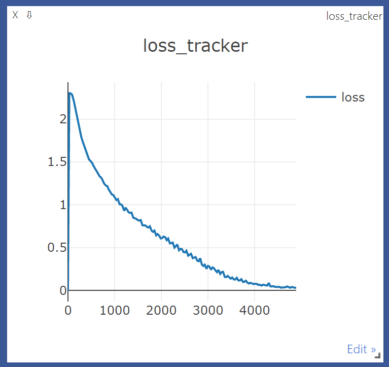
저번에 다뤘었던 visdom을 이용하여 시각화를 하면서 학습을 진행한다.
Data
데이터는 CIFAR10를 이용하여 학습을 진행한다.
1
2
3
4
5
6
7
8
9
10
11
12
13
14
15
16
17
transform = transforms.Compose(
    [transforms.ToTensor(),
     transforms.Normalize((0.5, 0.5, 0.5), (0.5, 0.5, 0.5))])

trainset = torchvision.datasets.CIFAR10(root='./cifar10', train=True,
                                        download=True, transform=transform)
trainloader = torch.utils.data.DataLoader(trainset, batch_size=512,
                                          shuffle=True, num_workers=0)

testset = torchvision.datasets.CIFAR10(root='./cifar10', train=False,
                                       download=True, transform=transform)

testloader = torch.utils.data.DataLoader(testset, batch_size=4,
                                         shuffle=False, num_workers=0)

classes = ('plane', 'car', 'bird', 'cat',
           'deer', 'dog', 'frog', 'horse', 'ship', 'truck')
데이터셋들을 불러 DataLoader를 통해 학습하기 용이하게 만들어준다.
1
2
3
4
5
6
7
8
9
10
11
12
13
14
import matplotlib.pyplot as plt
import numpy as np

# get some random training images
dataiter = iter(trainloader)
images, labels = dataiter.next()
vis.images(images/2 + 0.5)

# print labels
print(' '.join('%5s' % classes[labels[j]] for j in range(4)))

'''output
truck   dog horse truck
'''
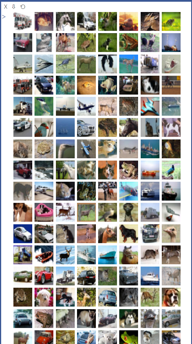
class와 이미지가 잘 받아진 것을 확인할 수 있다.
Model
1
2
3
4
5
6
7
8
9
10
11
12
13
14
15
16
17
18
19
20
21
22
23
24
25
26
27
28
29
30
31
32
33
34
35
36
37
38
39
40
41
42
43
import torchvision.models.vgg as vgg

cfg = [32,32,'M', 64,64,128,128,128,'M',256,256,256,512,512,512,'M'] #13 + 3 =vgg16

class VGG(nn.Module):

    def __init__(self, features, num_classes=1000, init_weights=True):
        super(VGG, self).__init__()
        self.features = features
        #self.avgpool = nn.AdaptiveAvgPool2d((7, 7))    -> 굳이 쓸 필요가 없음
        self.classifier = nn.Sequential(
            nn.Linear(512 * 4 * 4, 4096),
            nn.ReLU(True),
            nn.Dropout(),
            nn.Linear(4096, 4096),
            nn.ReLU(True),
            nn.Dropout(),
            nn.Linear(4096, num_classes),
        )
        if init_weights:
            self._initialize_weights()

    def forward(self, x):
        x = self.features(x)
        #x = self.avgpool(x)
        x = x.view(x.size(0), -1)
        x = self.classifier(x)
        return x

    def _initialize_weights(self):
        for m in self.modules():
            if isinstance(m, nn.Conv2d):
                nn.init.kaiming_normal_(m.weight, mode='fan_out', nonlinearity='relu')
                if m.bias is not None:
                    nn.init.constant_(m.bias, 0)
            elif isinstance(m, nn.BatchNorm2d):
                nn.init.constant_(m.weight, 1)
                nn.init.constant_(m.bias, 0)
            elif isinstance(m, nn.Linear):
                nn.init.normal_(m.weight, 0, 0.01)
                nn.init.constant_(m.bias, 0)

vgg16= VGG(vgg.make_layers(cfg),10,True).to(device)
앞서 정의했던 VGG16은 'D': [64, 64, 'M', 128, 128, 'M', 256, 256, 256, 'M', 512, 512, 512, 'M', 512, 512, 512, 'M']의 형태였는데 위의 모델은 조금 달라보인다. 이건 CIFAR10의 이미지가 32x32로 imgagenet의 것보다 작기 때문이다. 기존대로 pooling을 모두 진행하면 데이터의 크기가 너무 작아지므로 그것을 방지하기 위함이다.
같은 이유로 avgpool layer도 빠졌는데 기존의 max pooling만 해도 이미 7x7보다 크기가 작기 때문이다.
나머지는 모두 같은 방식으로 작성되었다.
1
2
3
4
5
6
7
8
a=torch.Tensor(1,3,32,32).to(device)
out = vgg16(a)
print(out)

'''output
tensor([[ 0.0125, -0.0020, -0.0270,  0.0210,  0.0100,  0.0126, -0.0009,  0.0242,
         -0.0099,  0.0185]], device='cuda:0', grad_fn=<AddmmBackward>)
'''
test했을 때도 문제가 없으므로 사용할 준비가 모두 되었다.
Optimizer and Loss
1
2
3
4
5
criterion = nn.CrossEntropyLoss().to(device)
optimizer = torch.optim.SGD(vgg16.parameters(), lr = 0.005,momentum=0.9)

# 학습이 진행됨에 따라 lr 조절
lr_sche = optim.lr_scheduler.StepLR(optimizer, step_size=5, gamma=0.9) # optimizer의 step이 5번 진행될 때마다 gamma만큼 곱함
기존과 다른 점은 학습된 정도에 따라 learning rate를 줄이는 코드가 추가되었다는 것이다.
Train
1
2
3
4
5
6
7
8
9
10
11
12
13
14
15
16
17
18
19
20
21
22
23
24
25
26
27
28
29
30
31
32
33
34
35
36
37
38
39
40
41
42
43
44
45
46
47
48
49
50
51
52
53
54
55
56
57
58
59
60
61
62
63
64
print(len(trainloader))
epochs = 50

for epoch in range(epochs):  # loop over the dataset multiple times
    running_loss = 0.0
    lr_sche.step()
    for i, data in enumerate(trainloader, 0):
        # get the inputs
        inputs, labels = data
        inputs = inputs.to(device)
        labels = labels.to(device)

        # zero the parameter gradients
        optimizer.zero_grad()

        # forward + backward + optimize
        outputs = vgg16(inputs)
        loss = criterion(outputs, labels)
        loss.backward()
        optimizer.step()

        # print statistics
        running_loss += loss.item()
        if i % 30 == 29:    # print every 30 mini-batches
            loss_tracker(loss_plt, torch.Tensor([running_loss/30]), torch.Tensor([i + epoch*len(trainloader) ]))
            print('[%d, %5d] loss: %.3f' %
                  (epoch + 1, i + 1, running_loss / 30))
            running_loss = 0.0


print('Finished Training')

'''output
98
[1,    30] loss: 2.302
[1,    60] loss: 2.299
[1,    90] loss: 2.284
[2,    30] loss: 2.208
[2,    60] loss: 2.128
[2,    90] loss: 2.068
[3,    30] loss: 1.974
[3,    60] loss: 1.856
[3,    90] loss: 1.793
[4,    30] loss: 1.727
[4,    60] loss: 1.678
[4,    90] loss: 1.626
[5,    30] loss: 1.571
[5,    60] loss: 1.529
[5,    90] loss: 1.513
[6,    30] loss: 1.487
[6,    60] loss: 1.452
[6,    90] loss: 1.429
[7,    30] loss: 1.387
[7,    60] loss: 1.363
[7,    90] loss: 1.333
[8,    30] loss: 1.314
[8,    60] loss: 1.284
[8,    90] loss: 1.248
...
[50,    30] loss: 0.034
[50,    60] loss: 0.030
[50,    90] loss: 0.030
Finished Training
'''
lr_sche.step()이 추가된 것 말고 크게 다른 점은 없다.
Test
1
2
3
4
5
6
7
8
9
10
11
12
13
14
15
16
17
18
19
20
correct = 0
total = 0

with torch.no_grad():
    for data in testloader:
        images, labels = data
        images = images.to(device)
        labels = labels.to(device)
        outputs = vgg16(images)

        _, predicted = torch.max(outputs.data, 1)

        total += labels.size(0)

        correct += (predicted == labels).sum().item()

print('Accuracy of the network on the 10000 test images: %d %%' % (
    100 * correct / total))

Accuracy of the network on the 10000 test images: 75 %
정확도는 75%로 나왔다.