모두를 위한 딥러닝 2 - Lab10-1: Convolution, Lab10-2: MNIST CNN
모두를 위한 딥러닝 Lab10-1: Convolution, Lab10-2: MNIST CNN 강의를 본 후 공부를 목적으로 작성한 게시물입니다.
Convolution
강의 자료에서는 ‘이미지(2차원 매트릭스) 위에서 stride 만큼 filter(kernel)을 이동시키면서 겹쳐지는 부분의 각 원소의 값을 곱해서 더한 값을 출력으로 하는 연산’이라고 나와있다. 자세히 어떤 과정의 연산인지 확인해 보자.
아래와 같이 차례대로 input, filter, output 행렬이 있다고 해보자.
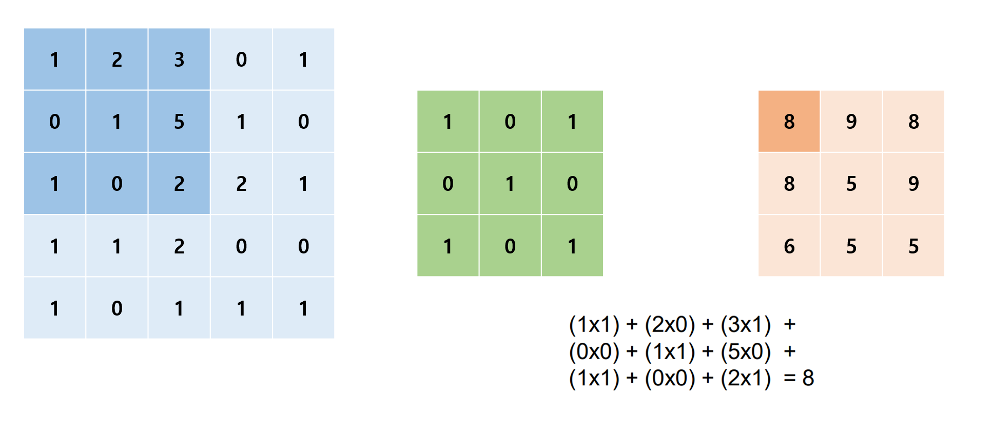
input, filter의 진한 부분을 각 자리끼리 곱해서 더해주는 것으로 output의 진한 부분의 결과를 낸다. 이 예제의 stride는 1이기 때문에 한 칸씩 커널을 이동하면서 이 과정을 진행하여 최종적으로 새로운 3x3 output을 만들어낸다.
우리가 원하는 filter와 stride를 설정하여 위 과정을 통해 새로운 매트릭스를 만드는 것이 convolution이다.
Padding
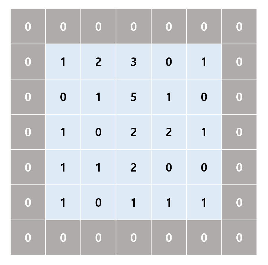
Convolution 연산에 쓰이는 데이터에 padding이라는 처리를 할 수 있는데, 이것은 input를 일정한 수로 감싼다는 뜻으로 1의 zero-padding을 한다는 것은 다음과 같은 입력으로 연산을 진행하겠다는 뜻이다.
Output Size
Convolution output의 크기는 다음과 같이 주어진다.
\[ Output \, size = \frac{input \, size - filter \, size + (2*padding)}{Stride} + 1 \]
예를 들어 input size = (32, 64), kernel = 5, stride = 1, padding = 0로 주어졌을 때
\[ (\frac{(32-5)+(0\times2)}{1}+1 , \frac{(32-5)+(0\times2)}{1}+1) = (28, 60) \]
위처럼 계산할 수 있다.
Input Type in PyTorch
PyTorch에서 torch.nn.Conv2d을 이용하여 convolution을 연산할 때 input data의 type은 torch.Tensor, shape은 (N x C x H x W) = (batch_size, channel, height, width)으로 맞춰줘야 한다.
위에서 size를 게산했던 예제를 실제로 코드로 실행하여 확인하려면 다음과 같이 작성하면 된다.
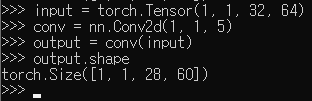
실제로도 계산 결과와 같은 shape이 나오는 것을 확인할 수 있다.
Convolution and Perceptron
convolution을 다음과 같이 perceptron으로 나타낼 수도 있다.
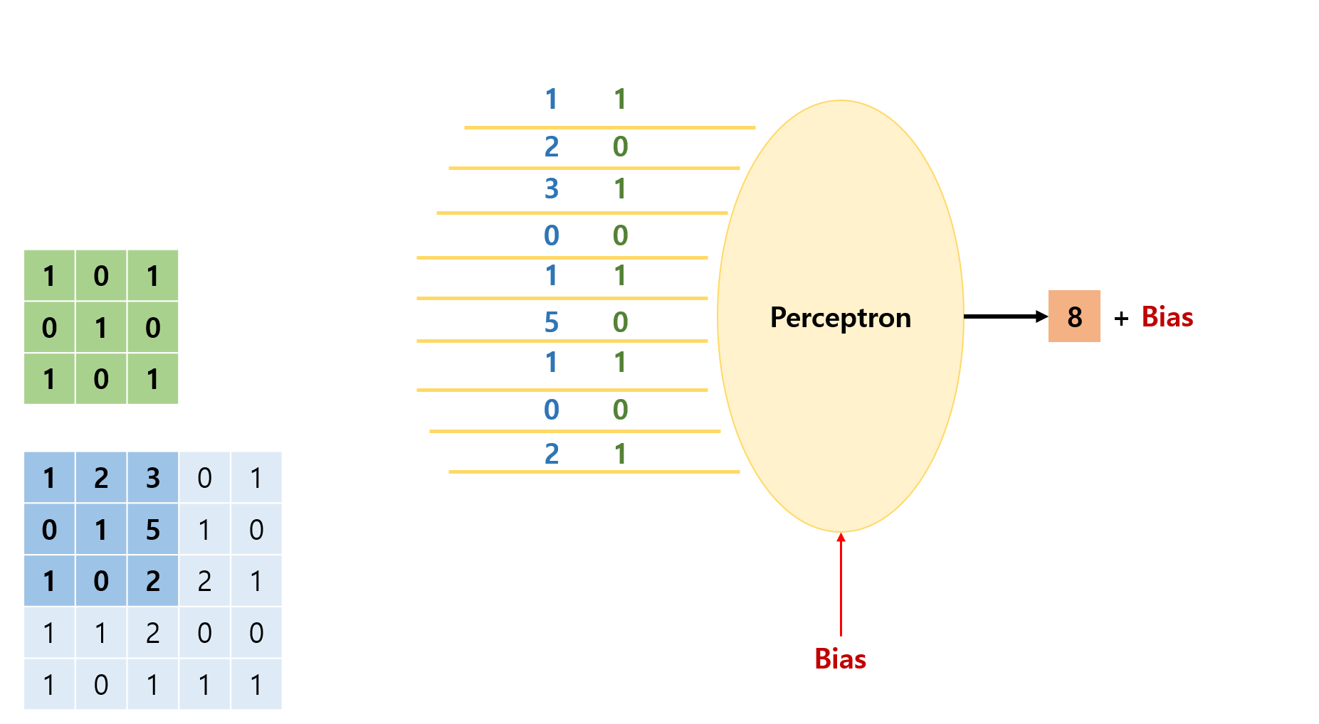
filter의 값을 weight로 가지고 있는 perceptron에 stride만큼 움직이면서 매트릭스를 통과시키면 output의 각 자리 결과값들이 계산된다.
Pooling
Pooling은 주어진 kernel size만큼의 구역을 대표하는 값들을 찾아서 그 대표값으로 새로운 매트릭스를 구성하는 것을 말한다.
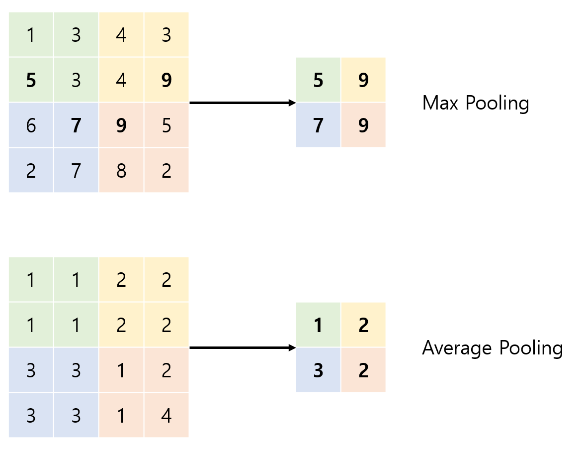
위 그림은 kernel size가 2인 max pooling과 average pooling을 나타낸 것이다.
max pooling은 그 구역의 최대값을 선택하는 것이고, average pooling은 평균값을 선택하여 새로운 매트릭스를 만드는 것이다.
Train CNN with MNIST
Import and Data
seed를 고정하고 mnist dataset을 불러와서 DataLoader를 적용하여 minibatch로 학습할 수 있도록 만들어 준다.
1
2
3
4
5
6
7
8
9
10
11
12
13
14
15
16
17
18
19
20
21
22
23
24
25
26
27
28
29
30
31
32
import torch
import torchvision.datasets as dsets
import torchvision.transforms as transforms
import torch.nn.init

device = 'cuda' if torch.cuda.is_available() else 'cpu'

# for reproducibility
torch.manual_seed(777)
if device == 'cuda':
    torch.cuda.manual_seed_all(777)

learning_rate = 0.001
training_epochs = 15
batch_size = 100

# MNIST dataset
mnist_train = dsets.MNIST(root='MNIST_data/',
                          train=True,
                          transform=transforms.ToTensor(),
                          download=True)

mnist_test = dsets.MNIST(root='MNIST_data/',
                         train=False,
                         transform=transforms.ToTensor(),
                         download=True)

# dataset loader
data_loader = torch.utils.data.DataLoader(dataset=mnist_train,
                                          batch_size=batch_size,
                                          shuffle=True,
                                          drop_last=True)
Model and Loss/Optimizer
이전과 다르게 3개의 큰 layer로 나누어 model을 생성한다. 2개의 convolution layer를 통과하고 하나의 fully connected layer를 통과시킨다. 단, fully connected layer로 들어가기 전에 linear layer에 들어갈 수 있도록 data를 view를 이용하여 flat하게 만든다.
1
2
3
4
5
6
7
8
9
10
11
12
13
14
15
16
17
18
19
20
21
22
23
24
25
26
27
28
29
30
class CNN(torch.nn.Module):

    def __init__(self):
        super(CNN, self).__init__()
        # L1 ImgIn shape=(?, 1, 28, 28)
        #    Conv     -> (?, 32, 28, 28)
        #    Pool     -> (?, 32, 14, 14)
        self.layer1 = torch.nn.Sequential(
            torch.nn.Conv2d(1, 32, kernel_size=3, stride=1, padding=1),
            torch.nn.ReLU(),
            torch.nn.MaxPool2d(kernel_size=2, stride=2))
        # L2 ImgIn shape=(?, 32, 14, 14)
        #    Conv      ->(?, 64, 14, 14)
        #    Pool      ->(?, 64, 7, 7)
        self.layer2 = torch.nn.Sequential(
            torch.nn.Conv2d(32, 64, kernel_size=3, stride=1, padding=1),
            torch.nn.ReLU(),
            torch.nn.MaxPool2d(kernel_size=2, stride=2))
        # Final FC 7x7x64 inputs -> 10 outputs
        self.fc = torch.nn.Linear(7 * 7 * 64, 10, bias=True)
        torch.nn.init.xavier_uniform_(self.fc.weight)

    def forward(self, x):
        out = self.layer1(x)
        out = self.layer2(out)
        out = out.view(out.size(0), -1)   # Flatten them for FC
        out = self.fc(out)
        return out

model = CNN().to(device)
loss는 cross entropy를 사용하고 optimizer는 Adam을 사용한다. loss를 to(device)로 학습에 사용할 device에 붙여주고, optimizer를 생성할 때 model.parameters()를 넣어주는 것을 잊지 말자
1
2
criterion = torch.nn.CrossEntropyLoss().to(device)
optimizer = torch.optim.Adam(model.parameters(), lr=learning_rate)
Train
기존에 minibatch로 학습하던 코드와 크게 다를 것이 없다.
1
2
3
4
5
6
7
8
9
10
11
12
13
14
15
16
17
18
19
20
21
22
23
24
25
26
27
28
29
30
31
32
33
34
35
36
37
38
39
40
41
42
43
# train my model
total_batch = len(data_loader)
print('Learning started. It takes sometime.')
for epoch in range(training_epochs):
    avg_cost = 0

    for X, Y in data_loader:
        # image is already size of (28x28), no reshape
        # label is not one-hot encoded
        X = X.to(device)
        Y = Y.to(device)

        optimizer.zero_grad()
        hypothesis = model(X)
        cost = criterion(hypothesis, Y)
        cost.backward()
        optimizer.step()

        avg_cost += cost / total_batch

    print('[Epoch: {:>4}] cost = {:>.9}'.format(epoch + 1, avg_cost))

print('Learning Finished!')

'''output
Learning started. It takes sometime.
[Epoch:    1] cost = 0.223892078
[Epoch:    2] cost = 0.0621332489
[Epoch:    3] cost = 0.0448851325
[Epoch:    4] cost = 0.0356322788
[Epoch:    5] cost = 0.0289768185
[Epoch:    6] cost = 0.0248806253
[Epoch:    7] cost = 0.0209558196
[Epoch:    8] cost = 0.0180539284
[Epoch:    9] cost = 0.0153525099
[Epoch:   10] cost = 0.0128902728
[Epoch:   11] cost = 0.0104844831
[Epoch:   12] cost = 0.0100922994
[Epoch:   13] cost = 0.00803675782
[Epoch:   14] cost = 0.00732926652
[Epoch:   15] cost = 0.00600952888
Learning Finished!
'''
convolution layer를 이용하여 model을 구성해도 학습이 잘 된 것을 확인할 수 있다.
1
2
3
4
5
6
7
8
9
10
11
12
13
# Test model and check accuracy
with torch.no_grad():
    X_test = mnist_test.test_data.view(len(mnist_test), 1, 28, 28).float().to(device)
    Y_test = mnist_test.test_labels.to(device)

    prediction = model(X_test)
    correct_prediction = torch.argmax(prediction, 1) == Y_test
    accuracy = correct_prediction.float().mean()
    print('Accuracy:', accuracy.item())

'''output
Accuracy: 0.9878999590873718
'''