모두를 위한 딥러닝 2 - Lab1: Tensor Manipulation
모두를 위한 딥러닝 Lab 1: Tensor Manipulation 강의를 본 후 공부를 목적으로 작성한 게시물입니다.
1. Vector, Matrix and Tensor
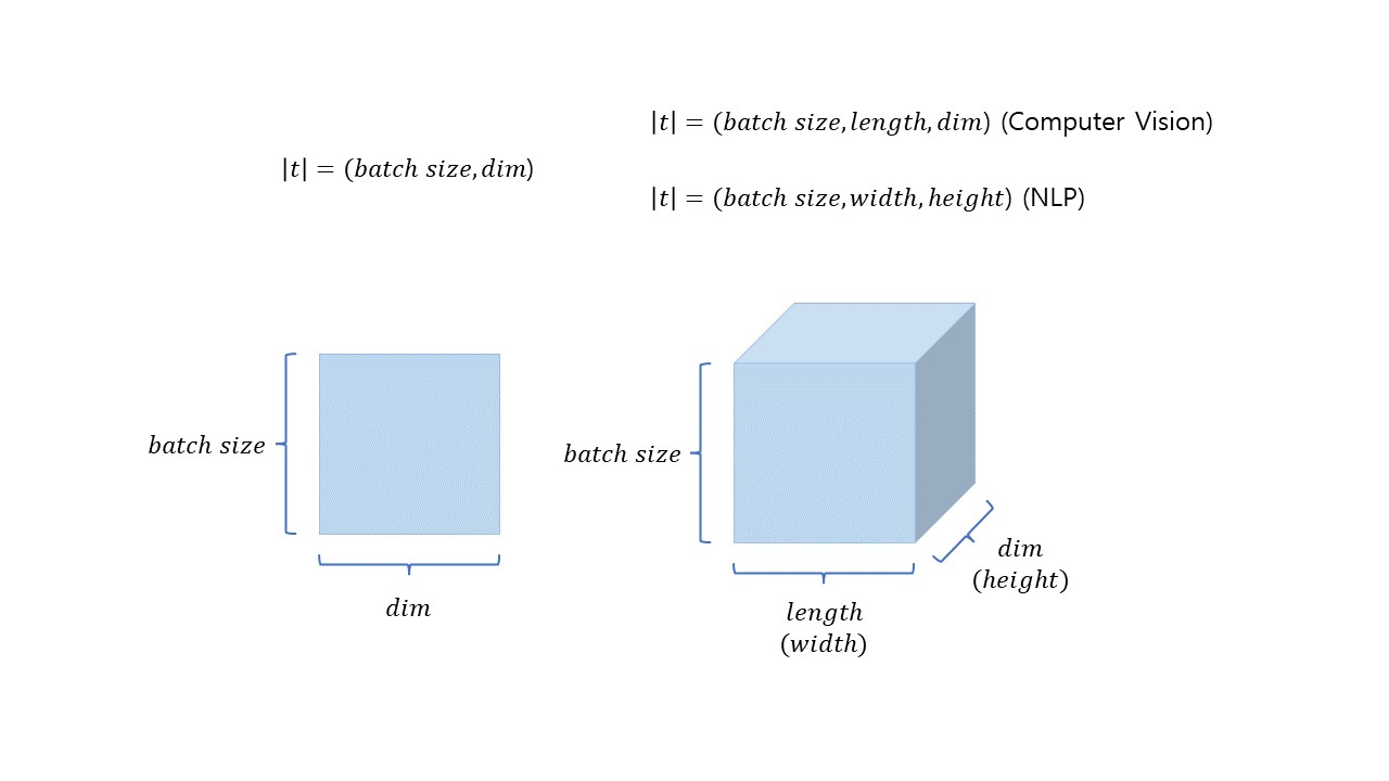
Vector, Matrix, Tensor의 표현은 위 그림과 같이 나타낼 수 있다.
각 구조들의 크기는 차원들의 크기의 곱으로 구할 수 있는데
Metrix와 Tonsor의 크기(t)는 위와 같이 구할 수 있다.
또한 위 그림의 차원의 순서는 파이토치에서 차원을 표현할 때의 순서와 같다. 즉, 아래와 같은 순서대로 표현하면 된다.
크기를 구할 때 봤던 순서를 다시 확인해 보면 Vector는 (batch size, dim)순, Tensor는 (batch size, length, dim)순으로 위 그림과 같은 순서로 표현한 것을 볼 수 있다.
Import
import numpy as np
import torch
2. Array with PyTorch
1D Array
t = torch.FloatTensor([0., 1., 2., 3., 4., 5., 6.])
print(t)

''' output
tensor([0., 1., 2., 3., 4., 5., 6.])
'''
1차원 배열의 경우 위와 같이 FloatTensor를 사용하여 배열을 PyTorch의 1차원 실수형 tensor로 변환할 수 있다.
2D Array
t = torch.FloatTensor([[1., 2., 3.],
                       [4., 5., 6.],
                       [7., 8., 9.],
                       [10., 11., 12.]
                      ])
print(t)

''' output
tensor([[ 1.,  2.,  3.],
        [ 4.,  5.,  6.],
        [ 7.,  8.,  9.],
        [10., 11., 12.]])
''''
2차원 배열의 경우에도 마찬가지로 FloatTensor를 사용하여 배열을 PyTorch의 2차원 실수형 tensor로 변환할 수 있다.
위 예제들에서는 실수형 tensor만을 예로 들었지만 다른 자료형들의 경우도 다음과 같이 tensor 생성이 가능하다.
각 type들에 대한 tensor 생성 방법은 다음과 같다.
# dtype: torch.float32 or torch.float (32-bit floating point)
torch.FloatTensor()

# dtype: torch.float64 or torch.double (64-bit floating point)
torch.FloatTensor()

# dtype: torch.uint8 (8-bit integer (unsigned))
torch.ByteTensor()

# dtype: torch.int8 (8-bit integer (signed))
torch.CharTensor()

# dtype: torch.int16 (16-bit integer (signed))
torch.ShortTensor()

# dtype: torch.int32 (32-bit integer (signed))
torch.IntTensor()

# dtype: torch.int64 (64-bit integer (signed))
torch.LongTensor()

# dtype: torch.bool
torch.BoolTensor()
위와 같이 타입을 지정하여 tensor를 생성해도 되지만 다음과 같이 생성할 수도 있다.
torch.tensor([[1., -1.], [1., -1.]])

''' output
tensor([[ 1.0000, -1.0000],
        [ 1.0000, -1.0000]])
'''
3. Frequently Used Operations in PyTorch
Broadcasting
서로 shape이 다른 tensor간의 연산을 할 때 자동으로 둘 중 더 작은 shape의 tensor를 더 shape이 큰 tensor의 shape으로 맞춰주어(broadcast) 계산해 주는 것을 말한다.
Same shape
m1 = torch.FloatTensor([[3, 3]])
m2 = torch.FloatTensor([[2, 2]])
print(m1 + m2)

''' output
tensor([[5., 5.]])
'''
같은 shape을 가지는 tensor 간의 연산은 위 코드의 결과처럼 같은 자리의 원소끼리 계산해 주면 된다.
Vector + Scalar
m1 = torch.FloatTensor([[1, 2]])
m2 = torch.FloatTensor([3]) # 3 -> [[3, 3]]
print(m1 + m2)

''' output
tensor([[4., 5.]])
'''
이번에는 vector와 scalar의 합이다. 이럴 때 [3]이 [[3, 3]]으로 boradcast 되어 shape을 동일하게 만든 후 연산을 진행하게 된다. 그래서 [[1, 2]] + [[3, 3]]의 결과인 [[4, 5]]가 나온다.
(2 x 1) Vector + (1 X 2) Vector
m1 = torch.FloatTensor([[1, 2]]) # [[1, 2]] -> [[1, 2], [1, 2]]
m2 = torch.FloatTensor([[3], [4]]) # [[3], [4]] -> [[3, 3], [4, 4]]
print(m1 + m2)

''' output
tensor([[4., 5.],
        [5., 6.]])
'''
서로 shape이 다른 vector간의 연산의 경우에도 작은 차원을 큰 차원으로 맞춘 후 연산을 한다.
위 코드에서는 [[1, 2]]이 [[1, 2], [1, 2]]로 [[3], [4]]가 [[3, 3], [4, 4]]로 각각 broadcast되어 연산을 진행하기 때문에 그 결과값은 [[4, 5], [5, 6]]이 나온다.
Mul vs. Matmul
둘다 tensor의 곱연산을 해 주며, 사용하는 형식도 m1.matmul(m2), m1.mul(m2)로 동일하지만 차이점은 앞서 언급한 broadcasting 여부에 있다.
# Without broadcasting
m1 = torch.FloatTensor([[1, 2], [3, 4]])
m2 = torch.FloatTensor([[1], [2]])
print('Shape of Matrix 1: ', m1.shape) # 2 x 2
print('Shape of Matrix 2: ', m2.shape) # 2 x 1
print(m1.matmul(m2)) # 2 x 1

# With broadcasting
m1 = torch.FloatTensor([[1, 2], [3, 4]])
m2 = torch.FloatTensor([[1], [2]])
print('Shape of Matrix 1: ', m1.shape) # 2 x 2
print('Shape of Matrix 2: ', m2.shape) # 2 x 1 ([[1], [2]]) -> 2 x 2 ([[1, 1], [2, 2]])
print(m1 * m2) # 2 x 2
print(m1.mul(m2))

''' output
Shape of Matrix 1:  torch.Size([2, 2])
Shape of Matrix 2:  torch.Size([2, 1])
tensor([[ 5.],
        [11.]])
Shape of Matrix 1:  torch.Size([2, 2])
Shape of Matrix 2:  torch.Size([2, 1])
tensor([[1., 2.],
        [6., 8.]])
tensor([[1., 2.],
        [6., 8.]])
'''matmul의 경우 broadcasting 없이 행렬 곱셈을 한다. 그러므로 각 tonsor의 shape 변화 없이 그대로 곱한다.
반면 mul은 broadcasting을 하고 행렬의 각 원소들을 곱한다. 이 때문에 m2의 shape이 2 x 1에서 2 x 2로 m1의 shape에 맞춰진 후에 각 자리의 원소끼리 곱셈이 계산된 것을 확인할 수 있다.
Mean
평균을 계산해 준다.
t = torch.FloatTensor([[1, 2], [3, 4]])
print(t)

''' output
tensor([[1., 2.],
        [3., 4.]])
'''

print(t.mean())
print(t.mean(dim=0)) # 첫 번째 차원 평균
print(t.mean(dim=1)) # 두 번째 차원 평균
print(t.mean(dim=-1)) # 마지막 차원 평균

''' output
tensor(2.5000)
tensor([2., 3.])
tensor([1.5000, 3.5000])
tensor([1.5000, 3.5000])
'''
매개변수로 dim을 입력할 수 있다. 아무것도 입력하지 않은 경우에는 tonsor에 포함된 값 전체를, 차원을 지정해 준 경우 그 차원의 값들로 평균을 계산하여 tensor를 반환한다.
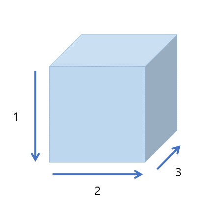
dim=0이면 첫 번째 차원(세로)을 기준으로 평균을 계산하고, dim=1이면 두 번째 차원(가로)을, dim=-1이면 마지막 차원(여기선 두 번째 차원)을 기준으로 평균을 계산한다.
Sum
합을 계산해 준다. 평균과 기본적으로 사용법이 같다. 차이점은 결과값으로 합을 반환한다는 것.
t = torch.FloatTensor([[1, 2], [3, 4]])
print(t)

''' output
tensor([[1., 2.],
        [3., 4.]])
'''

print(t.sum())
print(t.sum(dim=0)) # 첫 번째 차원 합
print(t.sum(dim=1)) # 두 번째 차원 합
print(t.sum(dim=-1)) # 마지막 차원 합

''' output
tensor(10.)
tensor([4., 6.])
tensor([3., 7.])
tensor([3., 7.])
'''
Max and Argmax
max는 최대값을 argmax는 최대값의 index를 의미한다.
t = torch.FloatTensor([[1, 2], [3, 4]])
print(t)

''' output
tensor([[1., 2.],
        [3., 4.]])
'''

print(t.max()) # Returns one value: max

''' output
tensor(4.)
'''
매개변수를 넣지 않으면 전체에서 최대값을 찾아 그 값을 반환한다.
print(t.max(dim=0)) # Returns two values: max and argmax (value amd index)
print('Max: ', t.max(dim=0)[0])
print('Argmax: ', t.max(dim=0)[1])

''' output
(tensor([3., 4.]), tensor([1, 1]))
Max:  tensor([3., 4.])
Argmax:  tensor([1, 1])
'''

print(t.max(dim=1))
print(t.max(dim=-1))

''' output
(tensor([2., 4.]), tensor([1, 1]))
(tensor([2., 4.]), tensor([1, 1]))
'''dim을 지정하면 해당 차원에서의 최대값과 그 차원에서 최대값의 위치를 tuple 형태로 반환한다.
위의 경우 dim=0(첫 번째 차원 - 열)을 기준으로 최대값인 3, 4와 그 값들의 index인 1, 1이 반환되는 것을 확인할 수 있다.
dim=1인 경우에도 기준이 되는 차원만 달라지고 같은 방식으로 (max, argmax)를 반환한다.
만약 argmax 값만 필요하다면 아래와 같이 torch.argmax()를 사용하여 값을 얻을 수 있다.
print(t.argmax(dim=0))
print(t.argmax(dim=1))
print(t.argmax(dim=-1))

''' output
tensor([1, 1])
tensor([1, 1])
tensor([1, 1])
'''
View
numpy의 reshape과 같은 역할을 한다.
t = np.array([[[0, 1, 2],
               [3, 4, 5]],

              [[6, 7, 8],
               [9, 10, 11]]])
ft = torch.FloatTensor(t)
print(ft.shape)

''' output
torch.Size([2, 2, 3])
'''

print(ft.view([-1, 3]))
print(ft.view([-1, 3]).shape)

''' output
tensor([[ 0.,  1.,  2.],
        [ 3.,  4.,  5.],
        [ 6.,  7.,  8.],
        [ 9., 10., 11.]])
'''

# -1은 보통 가장 변동이 심한 batch size 등(계산 실수가 많이 일어날 만한 곳)에 사용
# view(reshape) 하려는 결과 차원의 곱이 처음 차원들의 곱과 같아야 사용 가능
print(ft.view([-1, 1, 3]))
print(ft.view([-1, 1, 3]).shape)

''' output
tensor([[[ 0.,  1.,  2.]],

        [[ 3.,  4.,  5.]],

        [[ 6.,  7.,  8.]],

        [[ 9., 10., 11.]]])
'''
shape이 [2, 2, 3]인 tensor를 다른 shape들로 변경하는 예제이다.
이때 주의할 점은 shape을 변경할 대상과 변경한 후의 shape의 각 차원의 곱이 같아야 한다는 것이다. 위와 같이 shape이 [2, 2, 3]이라면 변경된 이후의 차원들의 곱도 2x2x3 = 12여야 한다.
많은 경우 위와 같이 한 차원에 -1을 넣어 차원을 자동으로 맞춰주도록 하는데, 보통 변동이 가장 심한 batch size 등에 -1을 적용하여 사용한다.
이렇게 사용하는 까닭은 변동이 심하거나 값이 큰 경우 매번 계산하는 것이 불편하기도 하고 계산하는 과정에서 실수가 발생할 수도 있기 때문이다.
Squeeze
걸레를 짜서 물을 빼내는 것과 같이 차원이 1인 것을 모두 삭제해 준다.
ft = torch.FloatTensor([[0], [1], [2]])
print(ft)
print(ft.shape)

''' output
tensor([[0.],
        [1.],
        [2.]])
torch.Size([3, 1])
'''

# 1이 있는 차원을 삭제
# dim=? 에 값을 넣을 경우 해당 차원이 1이면 삭제
print(ft.squeeze())
print(ft.squeeze().shape)

''' output
tensor([0., 1., 2.])
torch.Size([3])
'''
위와 같이 차원이 1아면 삭제해 준다. dim=?도 설정해 줄 수 있는데, 이 경우 해당 차원이 1이면 삭제한다. 예제와 같은 tensor의 경우 dim=1일 때 동일한 결과를 보여준다.
Unsqueeze
squeeze의 반대이다. 차원을 명시하여 그 차원을 1로 만들어 준다.
ft = torch.Tensor([0, 1, 2])
print(ft.shape)

''' output
torch.Size([3])
'''
# 차원(dim)을 명시하여 그 차원을 1로 만들어줌
print(ft.unsqueeze(0))
print(ft.unsqueeze(0).shape)

print(ft.unsqueeze(1))
print(ft.unsqueeze(1).shape)

''' output
tensor([[0., 1., 2.]])
torch.Size([1, 3])

tensor([[0.],
        [1.],
        [2.]])
torch.Size([3, 1])
'''
지정한 차원을 1로 만들어 주는 것을 볼 수 있다.
print(ft.view(1, -1))
print(ft.view(1, -1).shape)

print(ft.view(-1, 1))
print(ft.view(-1, 1).shape)

''' output
tensor([[0., 1., 2.]])
torch.Size([1, 3])

tensor([[0.],
        [1.],
        [2.]])
torch.Size([3, 1])
'''
view를 이용해서 같은 결과를 만들 수도 있다.
Casting
tensor의 형을 변환시켜주는 것을 말한다.
# 텐서의 형변환
t = torch.LongTensor([1, 2, 3, 4])
print(lt)

''' output
tensor([1, 2, 3, 4])
'''

print(lt.float())

''' output
tensor([1., 2., 3., 4.])
'''
위와 같이 tensor.float()으로 실수형 변환을 할 수 있고
bt = torch.ByteTensor([True, False, False, True])
print(bt)

''' output
tensor([1, 0, 0, 1], dtype=torch.uint8)
'''

print(bt.long())
print(bt.float())

''' output
tensor([1, 0, 0, 1])
tensor([1., 0., 0., 1.])
'''
이처럼 torch의 다른 타입들로도 변환이 가능하다.
Concatenation
tensor들을 이어붙인다.
x = torch.FloatTensor([[1, 2], [3, 4]])
y = torch.FloatTensor([[5, 6], [7, 8]])

# 주어진 차원이 늘어남 (이어 붙임)
print(torch.cat([x, y], dim=0))
print(torch.cat([x, y], dim=1))

''' output
tensor([[1., 2.],
        [3., 4.],
        [5., 6.],
        [7., 8.]])
tensor([[1., 2., 5., 6.],
        [3., 4., 7., 8.]])
'''
이 때 차원을 지정해 주면 그 차원으로 tensor를 잇는다. default는 dim=0
Stacking
cat과 비슷하지만 데이터의 차원은 유지하면서 쌓는다는 개념이 cat의 이어븥인다는 개념과는 조금 다르다.
x = torch.FloatTensor([1, 4])
y = torch.FloatTensor([2, 5])
z = torch.FloatTensor([3, 6])


print(torch.stack([x, y, z]))
print(torch.stack([x, y, z], dim=1))

''' output
tensor([[1., 4.],
        [2., 5.],
        [3., 6.]])
tensor([[1., 2., 3.],
        [4., 5., 6.]])
'''
마찬가지로 stack하는 방향을 dim으로 조절해 줄 수 있다.
또한, 이 과정은 unsqueeze와 cat의 조합으로 똑같이 진행할 수 있다.
# torch.cat([(1, 2), (1, 2), (1, 2)], dim=0) -> (3, 2) (stacking과 동일)
print(torch.cat([x.unsqueeze(0), y.unsqueeze(0), z.unsqueeze(0)], dim=0))

''' output
tensor([[1., 4.],
        [2., 5.],
        [3., 6.]])
'''
cat vs. stack
cat 과 stack이 조금 헷갈려서 차이점을 정리해볼까 한다.
결과값들의 shape을 비교해 보면 조금 더 차이점을 알기 쉽다.
x = torch.FloatTensor([[1, 2], [3, 4]])
y = torch.FloatTensor([[5, 6], [7, 8]])

print(x.shape, y.shape)
print(torch.cat([x, y], dim=0).shape)
print(torch.cat([x, y], dim=1).shape)

x = torch.FloatTensor([1, 4])
y = torch.FloatTensor([2, 5])
z = torch.FloatTensor([3, 6])

print(x.shape, y.shape, z.shape)
print(torch.stack([x, y, z]).shape)
print(torch.stack([x, y, z], dim=1).shape)

''' output
torch.Size([2, 2]) torch.Size([2, 2])
torch.Size([4, 2])
torch.Size([2, 4]

torch.Size([2]) torch.Size([2]), torch.Size([2]
torch.Size([3, 2])
torch.Size([2, 3])
'''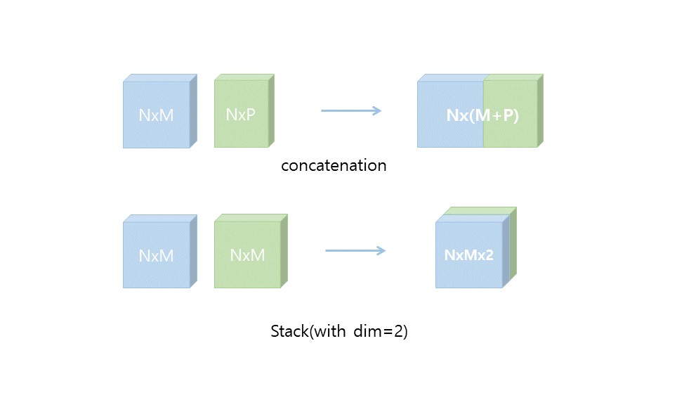
코드의 결과와 그림을 함께 보자.
concat의 경우 말 그대로 이어 붙이는 것이기 때문에 지정해 준 차원의 길이가 각 tensor의 차원 길이 만큼 늘어났다. 하지만 차원의 개수 변화는 없다. 반면, stack은 새로운 차원의 방향으로 쌓는 과정이기 때문에 tensor 간의 shape이 같아야 하고 차원이 하나 더 늘어난다. 그리고 그 차원의 크기는 쌓으려는 텐서의 개수와 같다.
다시 정리해 보면 conact은 데이터를 그대로 잇는 것, stack은 새로운 차원으로 쌓는 것이라는 차이점이 있다.
Ones and Zeros Like
해당 tensor와 같은 shape의 1 또는 0으로 채워진 tensor를 만든다.
x = torch.FloatTensor([[0, 1, 2], [2, 1, 0]])
print(x)

''' output
tensor([[0., 1., 2.],
        [2., 1., 0.]])
'''

# device도 같게 선언됨
print(torch.ones_like(x))
print(torch.zeros_like(x))

''' output
tensor([[1., 1., 1.],
        [1., 1., 1.]])
tensor([[0., 0., 0.],
        [0., 0., 0.]])
'''
이렇게 생성된 tensor는 shape 뿐만 아니라 device도 같게 생성된다. 즉, 바로 기존의 tensor와 연산이 가능하다.
In-place Operation
선언 없이 바로 결과값으로 대체한다. 사용법은 연산자에 _를 붙이면 된다.
print(x.mul(2.))
print(x)
# 선언 없이 바로 대체
print(x.mul_(2.))
print(x)

''' output
tensor([[2., 4.],
        [6., 8.]])
tensor([[1., 2.],
        [3., 4.]])
tensor([[2., 4.],
        [6., 8.]])
tensor([[2., 4.],
        [6., 8.]])
'''
선언하는 과정을 생략할 수 있다는 장점이 있지만 PyTorch의 gc가 잘 설계되어 있어서 속도면의 이점은 크게 없을 수도 있다고 한다.