카테고리: pytorch

"pytorch" 로 분류된 글.

MNIST = dsets.MNIST(root="./MNIST_data",train = True,transform=torchvision.transforms.ToTensor(), download=True)
cifar10 = dsets.CIFAR10(root="./cifar10",train = True, transform=torchvision.transforms.ToTensor(),download=True)

#CIFAR10
data = cifar10.__getitem__(0)
print(data[0].shape)
vis.images(data[0],env="main")

# MNIST
data = MNIST.__getitem__(0)
print(data[0].shape)
vis.images(data[0],env="main")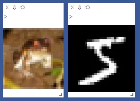

두꺼비(?)와 숫자 5가 잘 나온다. 또한 이런 이미지들도 당연히 vis.images()를 통해 한번에 많은 이미지도 출력할 수 있다.

Visdom

Visdom은 Meta 사(facebook)에서 제공하는 PyTorch에서 사용할 수 있는 시각화 도구이다. 실시간으로 데이터를 시각화하면서 바뀌는 점을 확인할 수 있다는 장점이 있다.

2022.05.22·8분·visdom

PYTORCHLAB 10-1

class CNN(torch.nn.Module):

    def __init__(self):
        super(CNN, self).__init__()
        # L1 ImgIn shape=(?, 1, 28, 28)
        #    Conv     -> (?, 32, 28, 28)
        #    Pool     -> (?, 32, 14, 14)
        self.layer1 = torch.nn.Sequential(
            torch.nn.Conv2d(1, 32, kernel_size=3, stride=1, padding=1),
            torch.nn.ReLU(),
            torch.nn.MaxPool2d(kernel_size=2, stride=2))
        # L2 ImgIn shape=(?, 32, 14, 14)
        #    Conv      ->(?, 64, 14, 14)
        #    Pool      ->(?, 64, 7, 7)
        self.layer2 = torch.nn.Sequential(
            torch.nn.Conv2d(32, 64, kernel_size=3, stride=1, padding=1),
            torch.nn.ReLU(),
            torch.nn.MaxPool2d(kernel_size=2, stride=2))
        # Final FC 7x7x64 inputs -> 10 outputs
        self.fc = torch.nn.Linear(7 * 7 * 64, 10, bias=True)
        torch.nn.init.xavier_uniform_(self.fc.weight)

    def forward(self, x):
        out = self.layer1(x)
        out = self.layer2(out)
        out = out.view(out.size(0), -1)   # Flatten them for FC
        out = self.fc(out)
        return out

model = CNN().to(device)

Convolution

강의 자료에서는 '이미지(2차원 매트릭스) 위에서 stride 만큼 filter(kernel)을 이동시키면서 겹쳐지는 부분의 각 원소의 값을 곱해서 더한 값을 출력으로 하는 연산'이라고 나와있다. 자세히 어떤 과정의 연산인지 확인해 보자.

2022.05.21·10분·convolution

PYTORCHLAB 9-4

# nn layers
linear1 = torch.nn.Linear(784, 32, bias=True)
linear2 = torch.nn.Linear(32, 32, bias=True)
linear3 = torch.nn.Linear(32, 10, bias=True)
relu = torch.nn.ReLU()
bn1 = torch.nn.BatchNorm1d(32)
bn2 = torch.nn.BatchNorm1d(32)

nn_linear1 = torch.nn.Linear(784, 32, bias=True)
nn_linear2 = torch.nn.Linear(32, 32, bias=True)
nn_linear3 = torch.nn.Linear(32, 10, bias=True)

# model with Batch normalization
bn_model = torch.nn.Sequential(linear1, bn1, relu,
                            linear2, bn2, relu,
                            linear3).to(device)

# model without Batch normalization
nn_model = torch.nn.Sequential(nn_linear1, relu,
                               nn_linear2, relu,
                               nn_linear3).to(device)

# define cost/loss & optimizer
criterion = torch.nn.CrossEntropyLoss().to(device)    # Softmax is internally computed.
bn_optimizer = torch.optim.Adam(bn_model.parameters(), lr=learning_rate)
nn_optimizer = torch.optim.Adam(nn_model.parameters(), lr=learning_rate)

Batch Normalization

Gradient Vanishing(기울기 소실)과 Gradient Exploding(기울기 폭주)는 정상적인 학습을 할 수 없게 만드는 요인들이다.

2022.05.14·6분·batch-normalization

PYTORCHLAB 9-3

model.train()    # set the model to train mode (dropout=True)
for epoch in range(training_epochs):
    avg_cost = 0

    for X, Y in data_loader:
        # reshape input image into [batch_size by 784]
        # label is not one-hot encoded
        X = X.view(-1, 28 * 28).to(device)
        Y = Y.to(device)

        optimizer.zero_grad()
        hypothesis = model(X)
        cost = criterion(hypothesis, Y)
        cost.backward()
        optimizer.step()

        avg_cost += cost / total_batch

    print('Epoch:', '%04d' % (epoch + 1), 'cost =', '{:.9f}'.format(avg_cost))

print('Learning finished')

'''output
Epoch: 0001 cost = 0.308392197
Epoch: 0002 cost = 0.142623395
Epoch: 0003 cost = 0.113427199
Epoch: 0004 cost = 0.093490042
Epoch: 0005 cost = 0.083772294
Epoch: 0006 cost = 0.077040948
Epoch: 0007 cost = 0.067025252
Epoch: 0008 cost = 0.063156039
Epoch: 0009 cost = 0.058766391
Epoch: 0010 cost = 0.055902217
Epoch: 0011 cost = 0.052059878
Epoch: 0012 cost = 0.048243146
Epoch: 0013 cost = 0.047231019
Epoch: 0014 cost = 0.045120358
Epoch: 0015 cost = 0.040942233
Learning finished
'''

Dropout

lab7-1에서 알아본 것처럼 학습을 하다보면 train set에 너무 과적합(overfitting)되는 경우가 발생한다.

2022.05.14·7분·dropout

PYTORCHLAB 9-2

# nn layers
linear1 = torch.nn.Linear(784, 256, bias=True)
linear2 = torch.nn.Linear(256, 256, bias=True)
linear3 = torch.nn.Linear(256, 10, bias=True)
relu = torch.nn.ReLU()

# xavier initialization
torch.nn.init.xavier_uniform_(linear1.weight) # not torch.nn.init.normal_()
torch.nn.init.xavier_uniform_(linear2.weight)
torch.nn.init.xavier_uniform_(linear3.weight)

'''output
Parameter containing:
tensor([[-0.0215, -0.0894,  0.0598,  ...,  0.0200,  0.0203,  0.1212],
        [ 0.0078,  0.1378,  0.0920,  ...,  0.0975,  0.1458, -0.0302],
        [ 0.1270, -0.1296,  0.1049,  ...,  0.0124,  0.1173, -0.0901],
        ...,
        [ 0.0661, -0.1025,  0.1437,  ...,  0.0784,  0.0977, -0.0396],
        [ 0.0430, -0.1274, -0.0134,  ..., -0.0582,  0.1201,  0.1479],
        [-0.1433,  0.0200, -0.0568,  ...,  0.0787,  0.0428, -0.0036]],
       requires_grad=True)
'''

Weight Initialization

초기 weight의 설정은 크게 중요하지 않아 보이지만 실제로는 큰 영향을 미친다. 위 그래프에서도 볼 수 있듯이 적절한 초기화 기법으로 초기화를 해준 경우(N이 붙어있는 곡선) 실제로 오차가 줄어든 것을 확인할 수 있다.

2022.05.13·6분·weight-init

PYTORCHLAB 9-1

criterion = torch.nn.CrossEntropyLoss().to(device)
optimizer = torch.optim.Adam(linear.parameters(), lr=learning_rate) # Adam optimizer

total_batch = len(data_loader)
for epoch in range(training_epochs):
    avg_cost = 0

    for X, Y in data_loader:
        # reshape input image into [batch_size by 784]
        # label is not one-hot encoded
        X = X.view(-1, 28 * 28).to(device)
        Y = Y.to(device)

        optimizer.zero_grad()
        hypothesis = linear(X)
        cost = criterion(hypothesis, Y)
        cost.backward()
        optimizer.step()

        avg_cost += cost / total_batch

    print('Epoch:', '%04d' % (epoch + 1), 'cost =', '{:.9f}'.format(avg_cost))

print('Learning finished')

'''output
Epoch: 0001 cost = 4.848181248
Epoch: 0002 cost = 1.464641452
Epoch: 0003 cost = 0.977406502
Epoch: 0004 cost = 0.790303528
Epoch: 0005 cost = 0.686833322
Epoch: 0006 cost = 0.618483305
Epoch: 0007 cost = 0.568978667
Epoch: 0008 cost = 0.531290889
Epoch: 0009 cost = 0.501056492
Epoch: 0010 cost = 0.476258427
Epoch: 0011 cost = 0.455025405
Epoch: 0012 cost = 0.437031567
Epoch: 0013 cost = 0.421489984
Epoch: 0014 cost = 0.408599794
Epoch: 0015 cost = 0.396514893
Learning finished
'''

ReLU

시그모이드 함수의 문제는 backpropagation과정에서 발생한다. backpropagation을 수행할 때 activation의 미분값 곱해가면서 사용하게 되는데 이때 기울기가 소실되는 gradient vanishing문제가 발생한다. 다음 그림은 시그모이드 함수

2022.05.13·8분·relu

PYTORCHLAB 8-2

linear1 = torch.nn.Linear(2, 10, bias=True)
linear2 = torch.nn.Linear(10, 10, bias=True)
linear3 = torch.nn.Linear(10, 10, bias=True)
linear4 = torch.nn.Linear(10, 1, bias=True)
sigmoid = torch.nn.Sigmoid()

model = torch.nn.Sequential(linear1, sigmoid, linear2, sigmoid, linear3, sigmoid, linear4, sigmoid).to(device)

for step in range(10001):
    optimizer.zero_grad()
    hypothesis = model(X)

    # cost/loss function
    cost = criterion(hypothesis, Y)
    cost.backward()
    optimizer.step()

    if step % 100 == 0:
        print(step, cost.item())

'''output
0 0.6948983669281006
100 0.6931558847427368
200 0.6931535005569458
300 0.6931513547897339
400 0.6931493282318115
500 0.6931473016738892
600 0.6931453943252563
700 0.6931434869766235
800 0.6931416988372803
900 0.6931397914886475
1000 0.6931380033493042
...
9700 0.00016829342348501086
9800 0.00016415018762927502
9900 0.00016021561168599874
10000 0.0001565046259202063
'''

Multi Layer Perceptron

MLP는 단일 퍼셉트론을 여러개 쌓은 것으로 단일 퍼셉트론으로 해결하지 못한 XOR과 같은 문제를 해결하기 위해 제안된 구조이다.

2022.05.12·7분·perceptron

PYTORCHLAB 8-1

linear = torch.nn.Linear(2, 1, bias=True)
sigmoid = torch.nn.Sigmoid()

# Sequential로 여러 모듈을 묶어 하나의 레이어로 사용
model = torch.nn.Sequential(linear, sigmoid).to(device)

criterion = torch.nn.BCELoss().to(device)
optimizer = torch.optim.SGD(model.parameters(), lr=1)

'''output
0 0.7273974418640137
100 0.6931475400924683
200 0.6931471824645996
300 0.6931471824645996
400 0.6931471824645996
500 0.6931471824645996
600 0.6931471824645996
...
9700 0.6931471824645996
9800 0.6931471824645996
9900 0.6931471824645996
10000 0.6931471824645996
'''

Perceptron

먼저 퍼셉트론의 컨셉이 된 뉴런에 대해 알아보자. 뉴런은 동물의 신경계를 구성하는 세포로 다음과 같은 형태이다.

2022.05.11·5분·perceptron

PYTORCHLAB 7-2

# MNIST data image of shape 28 * 28 = 784
linear = torch.nn.Linear(784, 10, bias=True).to(device)

# define cost/loss & optimizer
criterion = torch.nn.CrossEntropyLoss().to(device)
optimizer = torch.optim.SGD(linear.parameters(), lr=0.1)

모델은 선형모델을 사용하며 이미지의 크기가 28x28이므로 28*28=784의 차원을 가지는 입력을 받도록 정의한다.

for epoch in range(training_epochs):
    avg_cost = 0
    total_batch = len(data_loader)

    for X, Y in data_loader:
        # reshape input image into [batch_size by 784]
        # label is not one-hot encoded
        X = X.view(-1, 28 * 28).to(device)
        Y = Y.to(device)

        hypothesis = linear(X)
        cost = criterion(hypothesis, Y)
        
        optimizer.zero_grad()
        cost.backward()
        optimizer.step()

        avg_cost += cost / total_batch

    print('Epoch:', '%04d' % (epoch + 1), 'cost =', '{:.9f}'.format(avg_cost))

print('Learning finished')

'''output
Epoch: 0001 cost = 0.535468459
Epoch: 0002 cost = 0.359274179
Epoch: 0003 cost = 0.331187516
Epoch: 0004 cost = 0.316578031
Epoch: 0005 cost = 0.307158142
Epoch: 0006 cost = 0.300180674
Epoch: 0007 cost = 0.295130163
Epoch: 0008 cost = 0.290851504
Epoch: 0009 cost = 0.287417084
Epoch: 0010 cost = 0.284379542
Epoch: 0011 cost = 0.281825215
Epoch: 0012 cost = 0.279800713
Epoch: 0013 cost = 0.277809024
Epoch: 0014 cost = 0.276154280
Epoch: 0015 cost = 0.274440825
Learning finished
'''

MNIST Introduction

MNIST 데이터 셋은 숫자 손글씨를 모아놓은 데이터 셋이다. 사람들이 적은 숫자들을 우체국에서 자동으로 처리하기 위해 만들어진 것이 이 셋의 시작점이라고 한다.

2022.05.10·7분·mnist